Chapter 12: Practice: Accelerate your RAG with caching, asynchronous and vector engines
Advanced 2 introduces several methods to improve the efficiency of the RAG system, including persistent storage, more efficient vector indexing, engineering optimization in actual projects, and model inference optimization. As a corresponding practical tutorial, this section will first introduce you to how to use LazyLLM to implement persistent storage of knowledge base, and then the course will introduce LazyLLM's custom index component. Here we will teach you step by step how to use LazyLLM to create and use a custom index for retrieval. At the same time, the course will introduce the basic use of the high-performance vector database Milvus, and how to quickly access Milvus in LazyLLM to achieve high-speed vector search. Further, the course will introduce the use of the vLLM framework in LazyLLM to accelerate model inference and the use of quantized models to reduce hardware requirements. (For practical experience related to model distillation, you can jump to Elective 4 to learn.)
Environment preparation and basic component definition
If Python is installed on your computer, please install lazyllm and necessary dependency packages through the following command. For more detailed preparations about the LazyLLM environment, please refer to the corresponding content in Lecture 2.
After successfully installing lazyllm, we define the following components: large model llm, vector model embedding_model, and rerank_model. These components will be frequently used in the following practical process. After this part is predefined, it will not be defined again later.
For developers with tight GPU resources, it is recommended that you use the online model throughout the process to quickly get started with development and lower the threshold for use. The online model is created as follows (Code Github link):
from lazyllm import OnlineChatModule, OnlineEmbeddingModule

DOUBAO_API_KEY = ""
DEEPSEEK_API_KEY = ""
QWEN_API_KEY = ""

#Online large model, DeepSeek-V3 is used here
llm = OnlineChatModule(
    source="deepseek",
    api_key=DEEPSEEK_API_KEY,
)

#Vector model, here select the bean bag vector model
embedding_model = OnlineEmbeddingModule(
    source="doubao",
    embed_model_name="doubao-embedding-large-text-240915",
    api_key=DOUBAO_API_KEY,
)

#Rearrangement model. The online rearrangement model only supports Qianwen and Zhipu. The Qianwen rearrangement model is used here.
rerank_model = OnlineEmbeddingModule(
    source="qwen",
    api_key=QWEN_API_KEY,
    type="rerank"
)
For some developers who want to use remote connection to connect vector models, they can use TrainableModule to connect the vector models.
import os
import lazyllm

os.environ['LAZYLLM_OPENAI_API_KEY'] = 'empty'
lazyllm.config.refresh()

embedding = lazyllm.TrainableModule('bge-m3').deploy_method(lazyllm.deploy.auto, url='http://10.119.16.84:8000/v1/')
res = embedding(['你好', 'hello'], model='bge-m3')
print(res)
For scenarios where GPU resources are relatively sufficient, or where model efficiency or concurrency requirements are high, it is recommended to use lazyllm’s built-in TrainableModule to implement local deployment of the model:
from lazyllm import TrainableModule, pipeline

llm = TrainableModule('internlm2-chat-20b', stream=True)
embedding_model = TrainableModule("bge-large-zh-v1.5")
rerank_model = TrainableModule("bge-reranker-large")

pipeline(llm, embedding_model, rerank_model).start()
1. Use vector database to implement persistent storage of knowledge base
Vector database is a database system specially used to store, manage and retrieve high-dimensional vector data. It is widely used in search engines, recommendation systems, computer vision and natural language processing and other fields. Different from traditional relational databases, vector databases can efficiently store high-dimensional vectors and use similarity retrieval and optimized indexing technologies to greatly improve the efficiency of large-scale vector searches. They are an important data storage and retrieval tool for current AI applications.
LazyLLM natively supports two open source vector databases, ChromaDB and Milvus, providing out-of-the-box vector storage and retrieval support. In actual use, users only need to configure the store_conf parameter in the Document definition stage and perform simple storage and retrieval configuration** to use these two databases to store the document-processed data locally, and load the data directly from the local when the next system starts, avoiding repeated entry of documents into the database and achieving persistent storage of the knowledge base. The implementation of using store_conf to configure Document storage is as follows:
document = lazyllm.Document(dataset_path='/path/to/your/document',
           embed=lazyllm.OnlineEmbeddingModule(),
           ...,
           store_conf=store_conf)
The parameter store_conf receives the storage configuration in the form of a dictionary. The type and kwargs parameters need to be passed in during configuration. The specific fields are explained as follows:
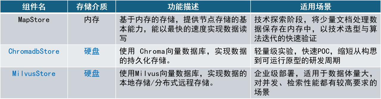
- type: Use storage type. As introduced before, the storage types currently supported by LazyLLM are map (based on memory), chroma (based on ChromaDB vector database) and milvus (based on Milvus vector database):
- map: Only use memory key/value storage to temporarily store all document processing data. The data will disappear after the system is restarted;
- chroma: Use ChromaDB to store data. ChromaDB is a lighter vector database. Compared with Milvus, the amount of data it can handle is limited and suitable for debugging. For more information about ChromoDB, please refer to ChromaDB official documentation;
- milvus: Use Milvus to store data, support the retrieval and storage of massive data, support distributed deployment, and are more suitable for production-level applications. For more information about Milvus, please refer to Milvus official documentation;
- kwargs: Additional configuration parameters required for specific storage, also entered in the form of a dictionary.
-

-
When type is chroma, the required configuration parameters are:
- dir (required): directory where data is stored;
- When type is milvus, the required configuration parameters are:
- uri (required): storage data address, which can be a file path or remote connection url;
- index_kwargs (optional): Index configuration of Milvus database, which can be a dict or list[dict]. The index configuration mainly contains two fields: index type index_type and metric type metric_type (i.e. Index and Similarity, very similar to the definition of LazyLLM). If the parameter is a dict, it means that all vector models use the same configuration; if you need to specify different vector models with different index configurations, you can pass it in in the form of a list, and embed_key can specify the configuration used. Currently, only floating point embedding and sparse embedding are supported. The parameters supported are as follows. Interested developers can go to the official website to view:
Practice 1 Use vector database to implement persistent storage
System startup performance comparison
In this part, while the other modules remain unchanged, memory, ChromaDB and Milvus are used as data storage respectively. The first and second startup times of the three were tested respectively to demonstrate the improvement of the efficiency of the secondary startup of the system by persistent storage. The file directory contains files in pdf, docx, and txt formats, with a total of 1614 nodes after being divided into blocks according to sentences.
- Memory storage
Since LazyLLM uses memory as the storage type by default, developers can define a Document that uses memory storage without any additional configuration:
- ChromaDB
ChromaDB is characterized by ease of use, high performance and tight integration of AI applications. It is suitable for application scenarios that require rapid deployment and lightweight management, such as chat robots, personalized recommendations, search engines, etc. Since ChromaDB implements persistent storage based on sqlite3, it does not support distributed deployment and is suitable for small local applications. ChromaDB using LazyLLM needs to configure the following fields in store_conf:
chroma_store_conf = {
  'type': 'chroma',
  'kwargs': {
'dir': 'dbs/test_chroma', # The dir passed in by chromadb is a folder. If it does not exist, it will be automatically created.
   }
}

document = lazyllm.Document(
    dataset_path='/path/to/your/document',
    embed=embedding_model,
    store_conf=chroma_store_conf
)
- Milvus
As an open source vector database designed for high-performance vector retrieval, Milvus can efficiently handle trillions of vector indexes. Compared with ChromaDB, Milvus not only provides vector storage, but also provides a high-speed retrieval interface, which can achieve efficient retrieval of vectors based on multiple indexing methods. To use Milvus as the storage backend, you need to pass in the following configuration:
milvus_store_conf = {
'type': 'milvus', # Specify the storage backend type
  'kwargs': {
'uri': 'test.db', # Store the backend address. This example uses the local file test.db. If the file does not exist, create a new file.
'index_kwargs': { # Storage backend index configuration
'index_type': 'FLAT', # Index type
'metric_type': 'COSINE', # Similarity calculation method
    }
  },
}

document = lazyllm.Document(
    dataset_path='/path/to/your/document',
    embed=embedding_model,
    store_conf=milvus_store_conf
)
Please note that currently LazyLLM supports Milvus 2.4.x, please note that your pymilvus >= 2.4.11, milvus-lite == 2.4.10.
When using Milvus, the retrieval will be based on the index configuration in the input configuration and the corresponding algorithm will be retrieved. There is no need to specify the similarity parameter in Retriever.
For a quick comparison, write the following test script to implement the performance test of the three stores (Code GitHub link):
import os
import time

import lazyllm
from lazyllm import LOG

from online_models import embedding_model # Use online models

DOC_PATH = os.path.abspath("docs") # General directory of practical documents

def test_store(store_conf: dict=None):
    """Receive storage configuration and test system startup performance under different configurations"""
    st1 = time.time()
    dataset_path = os.path.join(DOC_PATH, "test") # The path where the document is located

    docs = lazyllm.Document(
        dataset_path=dataset_path,
    embed=embedding_model, # Set embedding model
    store_conf=store_conf #Set storage configuration
        )
    docs.create_node_group(name='sentence', parent="MediumChunk", transform=lambda x: x.split('.')) # Create a node group

    if store_conf and store_conf.get('type') == "milvus":
# When the storage type is milvus, no similarity parameter is required
        retriever1 = lazyllm.Retriever(docs, group_name="sentence", topk=3)
    else:
# similariy=cosine to use vector retrieval
        retriever1 = lazyllm.Retriever(docs, group_name="sentence", similarity='cosine', topk=3)

    retriever1.start() # Start the retriever
    et1 = time.time()

# Test the time taken for a single retrieval
    st2 = time.time()
    res = retriever1("Chinatown")
    et2 = time.time()
    nodes = "\n======\n".join([node.text for node in res]) # Output the search results
    msg = f"Init time: {et1 - st1}, retrieval time: {et2 - st2}s\n" # Output system time
    LOG.info(msg)
    LOG.info(nodes)
    return msg

def test_stable_store():
    """Test multiple storage configurations at once"""
    chroma_store_conf = {
        'type': 'chroma',
        'kwargs': {
            'dir': 'dbs/chroma1',
        }
    }

    milvus_store_conf = {
        'type': 'milvus',
        'kwargs': {
            'uri': 'dbs/milvus1.db',
            'index_kwargs': {
            'index_type': 'HNSW',
            'metric_type': 'COSINE',
            }
        },
    }

    test_conf = {
        "map": None,
        "chroma": chroma_store_conf,
        "milvus": milvus_store_conf
    }
    start_times = ""
    for store_type, store_conf in test_conf.items():
        LOG.info(f"Store type: {store_type}")
        res = test_store(store_conf=store_conf)
        start_times += res
    print(start_times)

test_stable_store()
The running results are as follows:
| Storage type | First startup/retrieval time (s) | Second startup/retrieval time (s) |
|---|---|---|
| map | 17.71/0.36 | 17.30/0.36 |
| chroma | 17.69/0.37 | 13.89(↓21.5%)/0.36 |
| milvus | 15.30/0.02 | 1.80(↓88.2%)/0.02 |


According to the time-consuming data, we can see that due to performance errors when the system runs the program multiple times, using two vector databases to implement data persistence storage will improve system startup performance to varying degrees. When the system is started for the first time, the system initialization time of the three storage types is not much different, all at 16 to 17 seconds. However, when the system is started for the second time, the initialization time widens the gap. Among them, using ChromaDB has a small improvement in system startup efficiency, saving about 21% of the time. Using Milvus has greatly improved the system's secondary startup performance, saving about 87.36% of the startup time. It can be seen that using the storage backend can save time during the second startup of the system, and after using persistent storage, the system does not need to re-execute document blocking and document embedding, thereby saving a certain amount of computing resources.
Storage data management
LazyLLM provides a storage data management interface. By passing in manager=True or manager='ui' when creating a document, you can implement the addition, deletion, modification, and query functions of stored data.
import lazyllm

document = lazyllm.Document(dataset_path='/path/to/your/document',
                            embed=lazyllm.OnlineEmbeddingModule(),
                            store_conf=milvus_store_conf,
                            manager=True) # manager='ui'

document.start().wait()
doc_manager_url = document.manager.url
#doc_manager_url should be an address in the form http://127.0.0.1:12345/generate
# The valid part is http://127.0.0.1:12345
- manager=True
After starting the document management service, users can implement document management functions through a variety of interfaces, including querying documents, querying node groups, adding or updating documents, querying or updating document metadata, and other functions.
- manager='ui'
Provide a more intuitive interface to facilitate developers to view the group list, view the group file list, upload and delete files directly on the page. In both cases, users can add, delete, modify, and query documents through the interface. You can access the Swagger API interface document at http://127.0.0.1:12345/docs to obtain more detailed interface documentation. If you need to add or delete documents, you can perform specified operations through the http protocol. Specifically, document manager provides the following interfaces
API documentation GET /docs
List files GET /list_files
Upload files POST /upload_files
Add files POST /add_files
Delete files POST /delete_files
Add metafile POST /add_metadata
Delete meta information POST /delete_metadata_item
Add or update meta information /update_or_create_metadata_keys
Reset meta information /reset_metadata
Here is a simple example of uploading a file. You only need to splice the relevant URL from the API document:
import io
import json
import requests

doc_manager_url = '127.0.0.1:12345' # Change this to your url

# Get the number of documents in the document library
res = requests.get(f"http://{doc_manager_url}/list_files")
data = res.json().get('data')
# data is in the form
# [['36e494cd803e2eb0d04772a08277174ea13c1e9ba8a001c012def7437afc7d74',
#   'test.txt',
#   'file_path',
#   '2025-03-07 12:03:52',
#   '2025-03-07 12:03:52',
#   '{"docid": "36e494cd803e2eb0d04772a08277174ea13c1e9ba8a001c012def7437afc7d74",
#   "lazyllm_doc_path": "file_path"}',
#   'success',
#    1]]
print(len(data))

# Upload virtual document
# Here the document will be uploaded to the dataset_path path when Document is initialized.
# Note, just fill in the file name at the location of 'test1.txt'
files = [('files', ('test1.txt', io.BytesIO(b"file1 content"), 'text/plain')),
        ('files', ('test2.txt', io.BytesIO(b"file2 content"), 'text/plain'))]

# Parameters, override is set to true to overwrite the original document with the same name, metadatas are document meta information, you can upload it as needed
data = dict(override='true', metadatas=json.dumps([{"version": "v1.2"},{"version": "v1.3"}]), user_path='/path')
# Splice parameters into url
url = f"http://{doc_manager_url}/upload_files" + ('?' + '&'.join([f'{k}={v}' for k, v in data.items()]))
response = requests.post(url, files=files)

# Get the number of documents in the document library
res = requests.get(f"http://{doc_manager_url}:39598/list_files?details=False")
data = res.json().get('data')
print(len(data))
Assuming that the document library has only one file, the output of the above code should satisfy:
2. Build efficient index to improve retrieval performance
Before this lesson, we learned to create multi-node groups and use multi-path recall to optimize the retrieval effect. The addition of this strategy has higher requirements for the performance of the recall phase. In this section, we will show you the power of indexing through several sets of practices. We will teach you step by step how to use LazyLLM's custom index component to create an efficient index, use an efficient Milvus database from scratch, and use the Milvus database in the simplest way in LazyLLM. Finally, we will introduce you to some engineering optimization techniques in the RAG system (such as caching and parallel mechanisms), and comprehensively introduce to you how to improve the efficiency of the retrieval stage.
Practice 2 Build an efficient index and improve retrieval speed
According to the previous introduction, there are currently some indexes (Index) built into LazyLLM, such as DefaultIndex, _FileNodeIndex and SmartEmbeddingIndex. Among them, DefaultIndex is the default Index, which supports embedding and text types. It performs similarity calculation in order and returns topk nodes, that is, linear search. Linear search has high time complexity and is not suitable for retrieval of large data sets; _FileNodeIndex supports obtaining corresponding nodes through file; SmartEmbeddingIndex supports high-speed vector retrieval through the Milvus interface.
Let’s try our hand at building a dictionary tree using IndexBase
Since the built-in linear search retrieval efficiency of LazyLLM is low, this practice will introduce how to use LazyLLM to build a custom index and improve the speed of vector retrieval. In LazyLLM, all indexes are created using the IndexBase component, and then the index component can be registered in the Document and used in subsequent retrieval processes. Let's first take the dictionary lookup example in Lecture 11 and use IndexBase to create a dictionary tree to achieve efficient word query.
Index implementation
Creating a custom index using IndexBase requires implementing three methods: index update (update), node removal (remove), and retrieval (query). The dictionary tree is a multi-tree, and we create a dictionary tree index according to its definition (see GitHub link):
from typing import Dict, List, Optional

import lazyllm
from lazyllm.tools.rag import IndexBase, LazyLLMStoreBase, DocNode
from lazyllm.common import override

#Define dictionary tree nodes
class TrieNode:
    def __init__(self):
        self.children: Dict[str, TrieNode] = {} # The child node set key is a letter
        self.is_end_of_word: bool = False # Complete word mark
        self.uids: set[str] = set() # Save the complete word uid of the current node

class TrieTreeIndex(IndexBase):
    def __init__(self, store: 'LazyLLMStoreBase'):
        self.store = store # Bind storage
        self.root = TrieNode() # Define the root node
        self.uid_to_word: Dict[str, str] = {} # uid--word mapping relationship

    @override
    def update(self, nodes: List['DocNode']) -> None:
        if not nodes or nodes[0]._group != 'trie_tree':
            return
        # Create an index for each word
        for n in nodes:
            uid = n._uid
            word = n.text
            self.uid_to_word[uid] = word
            node = self.root
            # Iterate through each letter from the first letter of the word
            for char in word:
                # Get the child branch of the corresponding letter of the node
                node = node.children.setdefault(char, TrieNode())
            node.is_end_of_word = True
            node.uids.add(uid)

    @override
    def remove(self, uids: List[str], group_name: Optional[str] = None) -> None:
        """Remove word from index"""
        if group_name != 'trie_tree':
            return
        for uid in uids:
            word = self.uid_to_word.pop(uid, None)
            if not word:
                continue
            self._remove(self.root, word, 0, uid)

    def _remove(self, node: TrieNode, word: str, index: int, uid: str) -> bool:
        if index == len(word):
            if uid not in node.uids:
                return False
            node.uids.remove(uid)
            node.is_end_of_word = bool(node.uids)
            return not node.children and not node.uids
        char = word[index]
        child = node.children.get(char)
        if not child:
            return False
        should_delete = self._remove(child, word, index + 1, uid)
        if should_delete:
            del node.children[char]
            return not node.children and not node.uids
        return False

    @override
    def query(self, query: str, group_name: str, **kwargs) -> List[str]:
        node = self.root
        # Traverse each letter of the word in query and find whether the word exists from the dictionary tree
        for char in query:
            node = node.children.get(char)
            if node is None:
                return []
        return self.store.get_nodes(group_name=group_name, uids=list(node.uids)) if node.is_end_of_word else []
The above code defines a scalar index based on a dictionary tree. First, this class inherits from IndexBase. The update and remove methods are used to add and delete the index of the corresponding word. The query method is used to find whether the target word is included in the dictionary tree. If the word is included in the dictionary tree, the node corresponding to the word is returned.
Note: When using the default storage (memory storage), the update and deletion of nodes will automatically be associated with the update and deletion of Index.
Index Registration
After defining the Index component above, you need to register it into the LazyLLM framework. When registering, we register in the form of key-value.
from lazyllm.tools.rag import Document

# Register by instantiating the object
document = Document(dataset_path="dataset_path", manager=False)
# Here document.get_store() will be passed transparently to TrieTreeIndex. If the Index you define does not receive any data during initialization, there is no need to pass it in.
document.register_index("trie_tree", TrieTreeIndex, document.get_store())
In the above code, a Document object is first instantiated, and then the Index component is registered through the Document instantiation object. When registering, you need to specify a string type key, that is, the name of the registered index, here is "trie_tree", then the defined class TrieTreeIndex, and finally specify the required initialization parameters, which are the parameters that the init method of the custom Index class needs to receive. You can pass in any constant as an initialization parameter, or you can pass in document.get_store() or document.get_embed(), which are parameters provided by lazy initialization in Document, representing the storage instance and embedded model respectively. If there are no parameters, no values need to be passed in.
Index usage
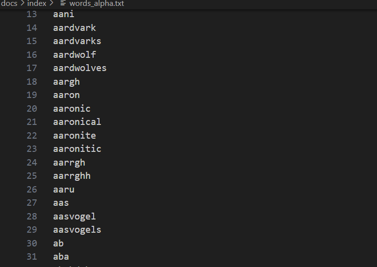
After defining and registering Index, it can be used in the retriever Retriever. We prepare a huge vocabulary list, which contains 370,000 English strings (mostly English words).
We also define a linear search index LinearIndex in the same way as above , note that this is only to show the performance difference between linear search and dictionary tree. In actual production, due to performance requirements, it is not recommended to use linear index for search. For the complete code, see link:
class LinearSearchIndex(IndexBase):
    def __init__(self):
        self.nodes = []

    @override
    def update(self, nodes: List['DocNode']) -> None:
        if not nodes or nodes[0]._group != 'linear':
            return
        for n in nodes:
            self.nodes.append(n)

    @override
    def remove(self, uids: List[str], group_name: Optional[str] = None) -> None:
        if group_name != 'linear':
            return
        for uid in uids:
            for i, n in enumerate(self.nodes):
                if n._uid == uid:
                    del self.nodes[i]
                    break

    @override
    def query(self, query: str, **kwargs) -> List[str]:
        # Assuming each word appears only once, only exact matching is performed
        res = []
        for n in self.nodes:
            if n.text == query:
                res.append(n)
                break
        return res
Define the index performance test program:
def test_trie_index(queries: list[str]):
    dataset_path = os.path.join(DOC_PATH, "index")
    docs1 = lazyllm.Document(dataset_path=dataset_path, embed=embedding_model)
    #Create node group
    docs1.create_node_group(name='linear', transform=(lambda d: d.split('\r\n')))
    docs1.create_node_group(name='tree', transform=(lambda d: d.split('\r\n')))
    # Register index
    docs1.register_index("trie_tree", TrieTreeIndex, docs1.get_store())
    docs1.register_index("linear_search", LinearSearchIndex)
    #Create a retriever and specify the corresponding index type
    retriever1 = lazyllm.Retriever(docs1, group_name="linear", index="linear_search", topk=1)
    retriever2 = lazyllm.Retriever(docs1, group_name="tree", index="trie_tree", topk=1)
    # Retrieval initialization
    retriever1.start()
    retriever2.start()
    for query in queries:
        st = time.time()
        res = retriever1(query)
        et = time.time()
        LOG.info(f"query: {query}, linear time: {et - st}, linear res: {res[0].text}")

        st = time.time()
        res = retriever2(query)
        et = time.time()
        LOG.info(f"query: {query}, trie time: {et - st}, trie res: {res[0].text}")

test_trie_index(["a", "lazyllm", "zwitterionic"])
Code running results:
query: a, linear time: 9.894371032714844e-05, linear res: a
query: a, trie time: 7.939338684082031e-05, trie res: a
query: lazyllm, linear time: 0.04016876220703125, linear res: lazyllm
query: lazyllm, trie time: 0.00011754035949707031, trie res: lazyllm
query: zwitterionic, linear time: 0.08771300315856934, linear res: zwitterionic
query: zwitterionic, trie time: 0.00011014938354492188, trie res: zwitterionic
It can be seen that both dictionary tree and linear search successfully search the corresponding nodes, but there is a clear difference in the time spent:
Linear search takes longer and longer as the search word goes further back in the vocabulary, while dictionary tree retrieval time is relatively stable. During the retrieval process of the last word in the 37w vocabulary list, the linear search took 0.0877s, and the dictionary tree only took 0.0001s, saving 99.89% of the time! Therefore, a properly designed index can greatly improve the retrieval efficiency of the system.
Combine the scenario and write the HNSW index yourself
In RAG scenarios, high-performance ANN vector indexes are often established to speed up vector retrieval. According to the introduction in the previous class, everyone has a certain understanding of HNSW. Next, we will also build an HNSW index according to the above idea of building an index, and compare the speed of vector retrieval in the case of LazyLLM's built-in cosine similarity + default index.
The implementation of HNSW index relies on the hnswlib library. One of the underlying ANN libraries of the popular vector database Milvus is hnswlib, which provides HNSW retrieval for milvus. The specific code is as follows (GitHub link):
class HNSWIndex(IndexBase):
def __init__(
self,
embed: Dict[str, Callable],
store: LazyLLMStoreBase,
max_elements: int = 10000, # Define the maximum index capacity
ef_construction: int = 200, # Balance index construction speed and search accuracy. The larger the index, the higher the accuracy but the slower the construction speed.
M: int = 16, # represents the number of edges of each vector during table construction. The higher M, the larger the memory usage, the higher the accuracy, and the slower the construction speed.
dim: int = 1024, # vector dimension
**kwargs
):
self.embed = embed
self.store = store
# Since the vector id in hnswlib cannot be str, a label is created to maintain the vector number.
# Create a dictionary to maintain the relationship between node id and vector id in hnsw
self.uid_to_label = {}
self.label_to_uid = {}
self.next_label = 0
#Initialize hnsw_index
self._index_init(max_elements, ef_construction, M, dim)
def _index_init(self, max_elements, ef_construction, M, dim):
# hnswlib supports multiple distance algorithms: l2, IP inner product and cosine
self.index = hnswlib.Index(space='cosine', dim=dim)
self.index.init_index(
max_elements=max_elements,
ef_construction=ef_construction,
M=M,
allow_replace_deleted=True
)
self.index.set_ef(100) # Set the maximum number of neighbors when searching. Higher values will lead to better accuracy, but the search speed will be slower.
self.index.set_num_threads(8) # Set the number of threads used during batch searches and index building processes
@override
def update(self, nodes: List['DocNode']):
if not nodes or nodes[0]._group != 'block':
return
# Node vectorization, here only the default embedding model is shown
parallel_do_embedding(self.embed, [], nodes=nodes, group_embed_keys={'block': ["__default__"]})
vecs = [] # vector list
labels = [] # vector id list
for node in nodes:
uid = str(node._uid)
# Record the relationship between uid and label. If it is a new uid, write next_label
if uid in self.uid_to_label:
label = self.uid_to_label[uid]
else:
label = self.next_label
self.uid_to_label[uid] = label
self.next_label += 1
# Get the default embedding result
vec = node.embedding['__default__']
vecs.append(vec)
labels.append(label)
self.label_to_uid[label] = uid
# Create hnsw index based on vector
data = np.vstack(vecs)
ids = np.array(labels, dtype=int)
self.index.add_items(data, ids)
@override
def remove(self, uids, group_name=None):
"""
Mark and delete a batch of vectors corresponding to uid and clean up the mapping
"""
if group_name != 'block':
return
for uid in map(str, uids):
if uid not in self.uid_to_label:
continue
label = self.uid_to_label.pop(uid)
self.index.mark_deleted(label)
self.label_to_uid.pop(label, None)
@override
def query(
self,
query: str,
topk: int,
embed_keys: List[str],
**kwargs,
) -> List['DocNode']:
# Generate query vector
parts = [self.embed[k](query) for k in embed_keys]
qvec = np.concatenate(parts)
#Call hnsw knn_query method for vector retrieval
labels, distances = self.index.knn_query(qvec, k=topk, num_threads=self.index.num_threads)
results = []
#Get retrieval topk
for lab, dist in zip(labels[0], distances[0]):
uid = self.label_to_uid.get(lab)
results.append(uid)
if len(results) >= topk:
break
# Get the node corresponding to uid from store
return self.store.get_nodes(group_name='block', uids=results) if len(results) > 0 else []
def test_hnsw_index():
dataset_path = os.path.join(DOC_PATH, "test")
docs1 = lazyllm.Document(dataset_path=dataset_path, embed=embedding_model)
docs1.create_node_group(name='block', transform=(lambda d: d.split('\n')))
docs1.register_index("hnsw", HNSWIndex, docs1.get_embed(), docs1.get_store())
retriever1 = lazyllm.Retriever(docs1, group_name="block", similarity="cosine", topk=3)
retriever2 = lazyllm.Retriever(docs1, group_name="block", index="hnsw", topk=3)
retriever1.start()
retriever2.start()
q = "Securities regulation?"
st = time.time()
res = retriever1(q)
et = time.time()
context_str = "\n---------\n".join([r.text for r in res])
LOG.info(f"query: {q}, default time: {et - st}, default res:\n {context_str}")
st = time.time()
res = retriever2(q)
et = time.time()
context_str = "\n---------\n".join([r.text for r in res])
LOG.info(f"query: {q}, HNSW time: {et - st}, HNSW res: \n{context_str}")
test_hnsw_index()
The running results are as follows:
query: Securities regulation? , default time: 0.5182957649230957, default res:
Protective measures from financial regulatory authorities
---------
In order to standardize the capital account management of securities companies, prevent business risks, and protect the legitimate rights and interests of customers, in accordance with the "China
---------
In order to implement the "Measures for the Administration of Securities Brokerage Business" and guide securities companies to carry out securities brokerage business in a standardized manner, we will coordinate
query: Securities regulation? , HNSW time: 0.021764516830444336, HNSW res:
Protective measures from financial regulatory authorities
---------
In order to implement the "Measures for the Administration of Securities Brokerage Business" and guide securities companies to carry out securities brokerage business in a standardized manner, we will coordinate
---------
In order to standardize the capital account management of securities companies, prevent business risks, and protect the legitimate rights and interests of customers, in accordance with the "China
It can be seen that using the default cosine similarity and default index to perform vector retrieval takes 0.518s, while using the self-implemented HNSW index to perform vector retrieval takes 0.022s, saving about 95% of the time. This conclusion is consistent with the practice of scalar indexing, that is, by establishing an efficient index and "exchanging space for time", the amount of calculation can be greatly reduced and the retrieval efficiency can be improved.
Practice 3: Start from scratch and use the high-performance vector database Milvus
Vector indexes are very powerful, but the cost of manually building a high-performance index from 0 is relatively high. If you are careful, you must have discovered that in the previous storage configuration, the configuration parameters of the Milvus vector database already include index-related configuration, that’s right! Vector databases have already indexed these high-performance vectors. In the actual research and development process, we only need to use these high-performance vector databases to achieve high-performance vector retrieval!
Introduction to the use of native Milvus
Let’s first take a look at the native basic usage of the high-performance vector database Milvus, the protagonist of this practice, including the installation of milvus and the use of basic functions (initialization, data injection, data retrieval).
Install
In this practice, we use Milvus Lite, a python library included in pymilvus that can be embedded into applications. Milvus also supports deployment on Docker and Kubernetes, making it suitable for production use cases. Run the following command to complete the installation of pymilvus.
use
First we use the following code to create a milvus client.
from pymilvus import MilvusClient
# Create a milvus client and pass in the storage path of the local database. If the path does not exist, create it.
client = MilvusClient("dbs/origin_milvus.db")
In Milvus, we need a Collections to store vectors and their associated metadata. It is equivalent to a table in a traditional SQL database. When creating Collections, you can define Schema and index parameters to configure vector specifications, such as dimension (dimension), index type (index_params), distance metric (metric_type), etc. Code GitHub link.
# In the initialization phase, if a collection with the same name already exists, delete it first
if client.has_collection(collection_name="demo_collection"):
    client.drop_collection(collection_name="demo_collection")

client.create_collection(
    collection_name="demo_collection",
    dimension=1024,
)
Note: create_collection supports more input parameters, such as primary key column name primary_field_name, vector column name vector_field_name, vector index parameter index_params, similarity parameter metric_type, etc. Only basic usage is introduced here, and the rest use default parameters.
Then prepare the document slices, vectorize them, create a data set according to the format accepted by milvus, and inject it into the database. Here we add an additional field subject (subject) to serve as the metadata of the data. Code GitHub link.
docs = [
    "Artificial intelligence was founded as an academic discipline in 1956.",
    "Alan Turing was the first person to conduct substantial research in AI.",
    "Born in Maida Vale, London, Turing was raised in southern England.",
]
vecs =[embedding_model(doc) for doc in docs]
data = [
    {"id": i, "vector": vecs[i], "text": docs[i], "subject": "history"}
    for i in range(len(vecs))
]
# Data injection
res = client.insert(collection_name="demo_collection", data=data)
print(f"Inserted data into client:\n {res}")
When performing query retrieval, you also need to vectorize the query first, then call the search method in the client, specify the corresponding collection and retrieval quantity, and support specifying which fields to output (output_fields). Code GitHub link.
query = "Who is Alan Turing?"
# query vectorization
q_vec = embedding_model(query)
# Retrieve
res = client.search(
collection_name="demo_collection", # Specify collection
    data=[q_vec],
limit=2, # Specify the number of searches (top_k)
output_fields=["text", "subject"], #Specify the fields included in the search results
)
print(f"Query: {query} \nSearch result:\n {res}")
Milvus not only supports simple and efficient vector retrieval, but also supports the use of metadata as filter fields to achieve consistent retrieval of scalar index + vector index. In the code below, we also create three paragraphs and set the subject to different subjects during data injection. In the input parameters of the search method, we enter the filter parameter to set the data we want to filter. Code GitHub link.
docs = [
    "Machine learning has been used for drug design.",
    "Computational synthesis with AI algorithms predicts molecular properties.",
    "DDR1 is involved in cancers and fibrosis.",
]
vecs =[embedding_model(doc) for doc in docs]
data = [
    {"id": 3 + i, "vector": vecs[i], "text": docs[i], "subject": "biology"}
    for i in range(len(vecs))
]
client.insert(collection_name="demo_collection", data=data)
res = client.search(
    collection_name="demo_collection",
    data=[embedding_model("tell me AI related information")],
filter="subject == 'biology'", # Fields expected to be filtered
    limit=2,
    output_fields=["text", "subject"],
)
print(f"Filter Query: {query} \nSearch result:\n {res}")
We combine the above usage methods and other components of LazyLLM to rebuild a simple RAG system (Code GitHub link):
import os

import lazyllm
from lazyllm.tools.rag import SimpleDirectoryReader, SentenceSplitter
from lazyllm.tools.rag.doc_node import MetadataMode

from pymilvus import MilvusClient

from online_models import embedding_model, llm, rerank_model

DOC_PATH = os.path.abspath("docs")

###################### File storage ##################################
# milvus client initialization
client = MilvusClient("dbs/rag_milvus.db")
if client.has_collection(collection_name="demo_collection"):
    client.drop_collection(collection_name="demo_collection")

client.create_collection(
    collection_name="demo_collection",
    dimension=1024,
)

#Load local files and parse -- block slicing -- vectorization -- storage
dataset_path = os.path.join(DOC_PATH, "test")
docs = SimpleDirectoryReader(input_dir=dataset_path)()
block_transform = SentenceSplitter(chunk_size=256, chunk_overlap=25)

nodes = []
for doc in docs:
    nodes.extend(block_transform(doc))

# Slice vectorization
vecs = [embedding_model(node.get_text(MetadataMode.EMBED)) for node in nodes]
data = [
    {"id": i, "vector": vecs[i], "text": nodes[i].text}
    for i in range(len(vecs))
]
#Data injection
res = client.insert(collection_name="demo_collection", data=data)

###################### Search Q&A ##################################
query = "What are the basic specifications for securities management?"

# Retrieval and generation
prompt = 'You are a friendly AI Q&A assistant who needs to provide answers based on the given context and question. \
Answer the questions based on the following information:\
        {context_str} \n '
llm.prompt(lazyllm.ChatPrompter(instruction=prompt, extra_keys=['context_str']))

q_vec = embedding_model(query)
res = client.search(
    collection_name="demo_collection",
    data=[q_vec],
    limit=12,
    output_fields=["text"],
)

# Extract search results
contexts = [res[0][i].get('entity').get("text", "") for i in range(len(res[0]))]

# rearrange
rerank_res = rerank_model(text=query, documents=contexts, top_n=3)
rerank_contexts = [contexts[res[0]] for res in rerank_res]

context_str = "\n-------------------\n".join(rerank_contexts)

res = llm({"query": query, "context_str": context_str})
print(res)
In the above code, we first define the milvus client using the native usage method, and then use LazyLLM's own document parser to extract the document content, convert it into slices, vectorize it and inject it into the vector database. Then perform query retrieval, extract the retrieval content and perform reordering, and then give the large model to answer.
Using Milvus in LazyLLM
From the above practical content, it is not difficult to find that milvus can achieve persistent storage and strong retrieval performance. However, the way to use native milvus is indeed a bit complicated, and users need to spend a lot of money to learn how to use a vector database from scratch. This is somewhat "troublesome" for developers. Simply LazyLLM has perfectly adapted Milvus. As mentioned previously, you can easily connect milvus to the RAG system with simple storage and indexing backend configuration. The specific configuration method is to add an additional field 'indices' to the above-mentioned storage backend configuration store_conf. indices is a python dictionary, key is the name of the index type, and value is the parameter required by the index type. The specific configuration is as follows:
store_conf = {
    'type': 'map',
    'indices': {
        'smart_embedding_index': {
'backend': 'milvus', # Set the index to use the Milvus backend
              'kwargs': {
'uri': 'dbs/test.db', # Milvus data storage address
                  'index_kwargs': {
'index_type': 'HNSW', # Set the index type
'metric_type': 'COSINE', # Set the metric type
                }
            },
        },
    },
}
- key: 'smart_embedding_index' (use the built-in vector index of the milvus vector database to achieve efficient vector retrieval)
- values:
- 'backend': Index backend, currently only supports passing in 'milvus', the Milvus vector database is used.
- 'kwargs': Additional configuration items when selecting the corresponding index backend. When selecting milvus, the configuration items are consistent with the storage backend using milvus, which are uri and index_kwargs.
Milvus supports a variety of indexing methods. Generally speaking, floating-point indexes (that is, indexing dense vectors) have many usage scenarios and are suitable for semantic retrieval of large-scale data. Binary indexes and sparse indexes are suitable for smaller data sets and can ensure a higher recall rate. Each indexing method has a corresponding recommended measurement method. You can choose according to the following table according to your needs:
| Index mode | Concrete type | Measurement type |
|---|---|---|
| Floating point index | - Plane - IVF_FLAT - IVF_SQ8 - IVF_PQ - GPU_IVF_FLAT - GPU_IVF_PQ - HNSW - DISKANN |
- Euclidean distance (L2) - Inner product (IP) - Cosine similarity (COSINE) |
| Binary Index | - BIN_FLAT - BIN_IVF_FLAT |
- Jaccard (JACCARD) - HAMMING (HAMMING) |
| Sparse Index | - SPARSE_INVERTED_INDEX - SPARSE_WAND |
- Inner Product (IP) |
Based on the above milvus configuration, we use LazyLLM's built-in SmartEmbeddingIndex to implement Milvus index access, and also compare the retrieval speed with Retriever using the default index (for the complete code, see Github link):
import os
import time

import lazyllm
from lazyllm import LOG

from online_models import embedding_model

DOC_PATH = os.path.abspath("docs")

milvus_store_conf = {
    'type': 'map',
    'indices': {
        'smart_embedding_index': {
            'backend': 'milvus',
            'kwargs': {
                'uri': "dbs/test_map_milvus.db",
                'index_kwargs': {
                    'index_type': 'HNSW',
                    'metric_type': 'COSINE',
                }
            },
        },
    },
}
dataset_path = os.path.join(DOC_PATH, "test")

docs = lazyllm.Document(dataset_path=dataset_path, embed=embedding_model, store_conf=milvus_store_conf)

# Use default index
retriever1 = lazyllm.Retriever(docs, group_name="MediumChunk", topk=6, similarity="cosine")
# Use milvus built-in HNSW index
retriever2 = lazyllm.Retriever(docs, group_name="MediumChunk", topk=6, index='smart_embedding_index')
retriever1.start()
retriever2.start()

q = "Securities regulation?"
st = time.time()
res = retriever1(q)
et = time.time()
LOG.info(f"query: {q}, default time: {et - st}")

st = time.time()
res = retriever2(q)
et = time.time()
LOG.info(f"query: {q}, milvus time: {et - st}")
In the configuration of store_conf, the storage backend and index backend are two independent parts. However, if the storage type is milvus, since the index configuration information is already included in kwargs, there is no need to configure additional indices to implement built-in vector retrieval.
As you can see, when using Milvus, it is the same as using Milvus as a storage backend. Pass the index configuration indices into store_conf, and then specify index='smart_embedding_index' in Retriever. Compared with the native usage, using store_conf makes the use of vector database easier and the code more concise and readable. The results of running the program are as follows:
query: Securities regulation? , default time: 0.16447973251342773
query: Securities regulation? , milvus time: 0.02178812026977539
Using LazyLLM's built-in Milvus to perform retrieval saves approximately 86.75% of retrieval time compared to the default vector index. Using Milvus as the index backend, the code to build a RAG system based on the multi-embedding recall strategy is as follows. The code below shows how to use dense and sparse retrieval at the same time:
import lazyllm
from lazyllm import bind, deploy

milvus_store_conf = {
    'type': 'milvus',
    'kwargs': {
        'uri': "milvus.db",
        'index_kwargs': [
            {
                'embed_key': 'bge_m3_dense',
                'index_type': 'IVF_FLAT',
                'metric_type': 'COSINE',
            },
            {
                'embed_key': 'bge_m3_sparse',
                'index_type': 'SPARSE_INVERTED_INDEX',
                'metric_type': 'IP',
            }
        ]
    },
}

bge_m3_dense = lazyllm.TrainableModule('bge-m3')
bge_m3_sparse = lazyllm.TrainableModule('bge-m3').deploy_method((deploy.AutoDeploy, {'embed_type': 'sparse'}))
embeds = {'bge_m3_dense': bge_m3_dense, 'bge_m3_sparse': bge_m3_sparse}
document = lazyllm.Document(dataset_path='/path/to/your/document',
           embed=embeds,
           store_conf=milvus_store_conf)

document.create_node_group(name="block", transform=lambda s: s.split("\n") if s else '')
bge_rerank = lazyllm.TrainableModule("bge-reranker-large")

with lazyllm.pipeline() as ppl:
    with lazyllm.parallel().sum as ppl.prl:
        ppl.prl.retriever1 = lazyllm.Retriever(doc=document,
                         group_name="block",
                         embed_keys=['bge_m3_dense'],
                         topk=3)
        ppl.prl.retriever = lazyllm.Retriever(doc=document,
                         group_name="block",
                         embed_keys=['bge_m3_sparse'],
                         topk=3)
    ppl.reranker = lazyllm.Reranker(name='ModuleReranker',model=bge_rerank, topk=3) | bind(query=ppl.input)
    ppl.formatter = (
      lambda nodes, query: dict(
          context_str=[node.get_content() for node in nodes],
          query=query)
    ) | bind(query=ppl.input)

    ppl.llm = lazyllm.OnlineChatModule().prompt(lazyllm.ChatPrompter(instruction=prompt, extra_keys=['context_str']))
webpage = lazyllm.WebModule(ppl, port=23492).start().wait()
Combined with the storage configuration introduced previously, we will fully optimize the storage and indexing of the RAG system in Lecture 7 to comprehensively improve the execution efficiency of the system. The code is as follows (GitHub link):
import os

import lazyllm
from lazyllm import Reranker

from online_models import embedding_model, llm, rerank_model # Use online models

DOC_PATH = os.path.abspath("docs")

#milvus storage and index configuration
milvus_store_conf = {
    'type': 'milvus',
    'kwargs': {
        'uri': "dbs/milvus1.db",
        'index_kwargs': {
        'index_type': 'HNSW',
        'metric_type': 'COSINE',
        }
    }
}
dataset_path = os.path.join(DOC_PATH, "test")

# Define Document and pass in configuration to use milvus storage and retrieval
docs = lazyllm.Document(dataset_path=dataset_path, embed=embedding_model, store_conf=milvus_store_conf)
#Create sentence node group
docs.create_node_group(name='sentence', parent="MediumChunk", transform=(lambda d: d.split('。')))
#Create MediumChunk, sentence node group multi-channel recall,
retriever1 = lazyllm.Retriever(docs, group_name="MediumChunk", topk=6, index='smart_embedding_index')
retriever2 = lazyllm.Retriever(docs, group_name="sentence", target="MediumChunk", topk=6, index='smart_embedding_index')
retriever1.start()
retriever2.start()
#Create reranker
reranker = Reranker('ModuleReranker', model=rerank_model, topk=3)

prompt = 'You are a friendly AI Q&A assistant who needs to provide answers based on the given context and question. \
Answer the questions based on the following information:\
        {context_str} \n '
llm.prompt(lazyllm.ChatPrompter(instruction=prompt, extra_keys=['context_str']))

query = "What are the guidelines for securities management?"

nodes1 = retriever1(query=query)
nodes2 = retriever2(query=query)
rerank_nodes = reranker(nodes1 + nodes2, query)
context_str = "\n======\n".join([node.get_content() for node in rerank_nodes])
print(f"context_str: \n{context_str}")
res = llm({"query": query, "context_str": context_str})
print(res)
Milvus not only supports local db file links, but also supports access to remote server endpoints.
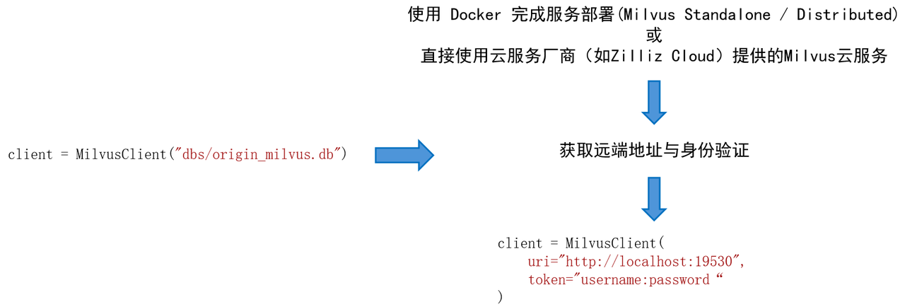
For example, we expect to deploy the Milvus Standalone service on a Linux system.
- Install Docker and check the hardware and software requirements according to Milvus official documentation.
- Install Milvus in Docker, installation script:
# Download the installation script
curl -sfL https://raw.githubusercontent.com/milvus-io/milvus/master/scripts/standalone_embed.sh -o standalone_embed.sh

# Start Docker container
bash standalone_embed.sh start
- Installation results:
- The docker container named Milvus is started on port 19530. To change the default configuration of Milvus, add the settings to the user.yaml file in the current folder and restart the service.
- Milvus data volumes are mapped to volumes/milvus in the current folder.
Practice 4 Engineering optimization skills, caching and parallel retrieval
In the previous Chapter 11, we mentioned some engineering optimization techniques, such as caching mechanism, multi-task parallelism, etc. Next we will practice respectively.
Use K-V cache
This practice uses a simple k-v dict to simulate the caching mechanism. We build a process from RAG system startup to retrieval, and set up the kv dictionary to save the retrieved query and node set, and test the retrieval time of the system with or without the caching mechanism:
Tips:
index='smart_embedding_index'has been abandoned in the latest lazyllm and needs to be changed tosimilarity='cosine'.
milvus_store_conf = {
    'type': 'map',
    'indices': {
        'smart_embedding_index': {
        'backend': 'milvus',
        'kwargs': {
            'uri': "dbs/test_cache.db",
            'index_kwargs': {
                'index_type': 'HNSW',
                'metric_type': 'COSINE',
            }
        },
        },
    },
}
dataset_path = os.path.join(DOC_PATH, "test")

docs = lazyllm.Document(
    dataset_path=dataset_path,
    embed=embedding_model,
    store_conf=milvus_store_conf
)
docs.create_node_group(name='sentence', parent="MediumChunk", transform=(lambda d: d.split('。')))

retriever1 = lazyllm.Retriever(docs, group_name="MediumChunk", topk=6, similarity='cosine')
retriever2 = lazyllm.Retriever(docs, group_name="sentence", target="MediumChunk", topk=6, similarity='cosine')
retriever1.start()
retriever2.start()

reranker = Reranker('ModuleReranker', model=rerank_model, topk=3)

# Set fixed query
query = "What are the basic specifications for securities management?"

# Run the retrieval process without caching mechanism 5 times and record the time
time_no_cache = []
for i in range(5):
    st = time.time()
    nodes1 = retriever1(query=query)
    nodes2 = retriever2(query=query)
    rerank_nodes = reranker(nodes1 + nodes2, query)
    et = time.time()
    t = et - st
    time_no_cache.append(t)
print(f"No cache The {i+1}th query takes time: {t}s")

# Define dict[list] to store the retrieved query and node collection to implement a simple caching mechanism
kv_cache = defaultdict(list)
for i in range(5):
    st = time.time()
#If the query is not in the cache, execute the normal retrieval process. If the query hits the cache, directly obtain the node set in the cache.
    if query not in kv_cache:
        nodes1 = retriever1(query=query)
        nodes2 = retriever2(query=query)
        rerank_nodes = reranker(nodes1 + nodes2, query)
# After the retrieval is completed, cache the query and retrieval nodes
        kv_cache[query] = rerank_nodes
    else:
        rerank_nodes = kv_cache[query]
    et = time.time()
    t = et - st
    time_no_cache.append(t)
print(f"KV cache {i+1} query time: {t}s")
The above code mainly implements the startup and retrieval links in the RAG system. For the retrieval link, the kv cache mechanism is implemented in the form of a dictionary. When the retrieval starts, it will first check whether the currently queried node is already in the cache. If it exists, it is a cache hit, and the query results in the cache can be directly fetched. Otherwise, the normal retrieval process will be carried out, and the retrieval results will be stored in the cache at the end. After running the program, you get the following output:
No cache The first query took: 1.3868563175201416s
No cache The second query took: 1.277320146560669s
No cache The third query took: 1.2744269371032715s
No cache The fourth query took: 1.3921117782592773s
No cache The fifth query took: 1.3207831382751465s
The first query of KV cache took 1.4092140197753906s
The second query of KV cache took: 2.384185791015625e-07s
The third query of KV cache took 1.430511474609375e-06s
The fourth query of KV cache took 2.384185791015625e-07s
The fifth query of KV cache took 2.384185791015625e-07s
It can be seen that when the system does not cache query results, the time of each query is 1. A few seconds, but when using cache, except for the first normal retrieval, all other retrievals are completed in an instant. Therefore, a reasonable design of the cache mechanism can further improve the system retrieval performance based on efficient vector indexing.
Note: The purpose of the practice is mainly to demonstrate the improvement of retrieval performance by the caching mechanism. In the actual production process, an in-memory data management system (such as Redis) is usually used to implement related functions. At the same time, many factors need to be considered to establish a complete caching mechanism. like:
- Document updates are cache cleansing
- Specific definition of high fever query
- Similar query hits
- ...
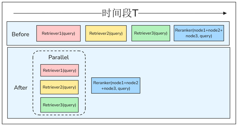
Parallel execution, multi-channel recall efficiency improvement
You can find that in the previous multi-channel recall scenario, the retrievers performed retrievals sequentially, which is actually very inefficient. Considering that there is no coupling between retrievers, we can use parallel in the Flow component of LazyLLM to implement parallel multi-way recall of retrievers.
The code is as follows:
milvus_store_conf = {
    'type': 'milvus',
    'kwargs': {
        'uri': "dbs/test_parallel.db",
        'index_kwargs': {
        'index_type': 'HNSW',
        'metric_type': 'COSINE',
        }
    }
}
dataset_path = os.path.join(DOC_PATH, "test")

docs1 = lazyllm.Document(
    dataset_path=dataset_path,
    embed=embedding_model,
    store_conf=milvus_store_conf
)
docs1.create_node_group(name='sentence', parent="MediumChunk", transform=(lambda d: d.split('。')))
retriever1 = lazyllm.Retriever(docs1, group_name="MediumChunk", topk=3)
retriever2 = lazyllm.Retriever(docs1, group_name="sentence", target="MediumChunk", topk=3)

retriever1.start()
retriever2.start()

with lazyllm.parallel().sum as prl:
    prl.r1 = retriever1
    prl.r2 = retriever2

query = "What are the basic specifications for securities management?"

st = time.time()
retriever1(query=query)
retriever2(query=query)
et1 = time.time()
prl(query)
et2 = time.time()
print(f"Sequential retrieval time: {et1-st}s")
print(f"Parallel retrieval time: {et2-et1}s")
Execute the above code to get the output:
It can be seen that using parallel retrieval can effectively save retrieval time and improve retrieval efficiency. Finally, we combine all the above optimization strategies to achieve a high-performance RAG system with optimized efficiency:
milvus_store_conf = {
    'type': 'milvus',
    'kwargs': {
        'uri': "dbs/test_rag.db",
        'index_kwargs': {
        'index_type': 'HNSW',
        'metric_type': 'COSINE',
        }
    }
}
dataset_path = os.path.join(DOC_PATH, "test")
#Define kv cache
kv_cache = defaultdict(list)

docs1 = lazyllm.Document(dataset_path=dataset_path, embed=embedding_model, store_conf=milvus_store_conf)
docs1.create_node_group(name='sentence', parent="MediumChunk", transform=(lambda d: d.split('。')))

prompt = 'You are a friendly AI Q&A assistant who needs to provide answers based on the given context and question. \
Answer the questions based on the following information: \
    {context_str} \n '

with lazyllm.pipeline() as recall:
# Parallel multi-way recall
    with lazyllm.parallel().sum as recall.prl:
        recall.prl.r1 = lazyllm.Retriever(docs1, group_name="MediumChunk", topk=6)
        recall.prl.r2 = lazyllm.Retriever(docs1, group_name="sentence", target="MediumChunk", topk=6)
    recall.reranker = lazyllm.Reranker(name='ModuleReranker',model=rerank_model, topk=3) | lazyllm.bind(query=recall.input)
    recall.cache_save = (lambda nodes, query: (kv_cache.update({query: nodes}) or nodes)) | lazyllm.bind(query=recall.input)

with lazyllm.pipeline() as ppl:
# Cache check
    ppl.cache_check = lazyllm.ifs(
        cond=(lambda query: query in kv_cache),
        tpath=(lambda query: kv_cache[query]),
        fpath=recall
    )
    ppl.formatter = (
        lambda nodes, query: dict(
            context_str="\n".join(node.get_content() for node in nodes),
            query=query)
    ) | lazyllm.bind(query=ppl.input)
    ppl.llm = llm.prompt(lazyllm.ChatPrompter(instruction=prompt, extra_keys=['context_str']))

w = lazyllm.WebModule(ppl, port=23492, stream=True).start().wait()
3. Use the vLLM framework to start the quantitative model service
vLLM is an efficient inference framework optimized specifically for large language model (LLM) inference. It aims to significantly improve the inference speed of large models and reduce graphics memory usage. It adopts a series of optimization technologies, such as efficient continuous batch processing (PagedAttention) and dynamic KV cache management, making it more advantageous than traditional methods in GPU inference scenarios.
1. Start the local service directly
LazyLLM natively supports three large model inference acceleration frameworks: LightLLM, LMDeploy and vLLM, and the Infinity embedded model acceleration framework. Users only need to specify the corresponding framework through TrainableModule.deploy_method when using it.
from lazyllm import TrainableModule, deploy

llm = TrainableModule('model_name').deploy_method(deploy.vllm)
vLLM supports inference services for most large models. You can first confirm whether the model you want to use is in the LazyLLM supported model list. The ones followed by AWQ, 4bit, etc. in this list are quantitative models. You can select a quantitative model according to your needs and start the dialogue service, for example
from lazyllm import TrainableModule, deploy

llm = TrainableModule('Qwen2-72B-Instruct-AWQ').deploy_method(deploy.vllm).start()
print(llm("hello, who are you?"))
Let's take Qwen2-72B-Instruct and its AWQ quantized version as an example to compare the size and running speed of the two. Running the Qwen2-72B-Instruct model of BF16 or FP16 requires at least 144GB of video memory (such as 2xA100-80G or 5xV100-32G); running the Int4 model requires at least 48GB of video memory (such as 1xA100-80G or 2xV100-32G), which is 33% of the original (data from Qwen Official [ModelScope Community]).

Let's briefly compare the running speed of the two (in a more rigorous case, you can compare the differences in multiple executions. For the complete code, see GitHub link):
import time
from lazyllm import TrainableModule, deploy, launchers

start_time = time.time()
llm = TrainableModule('Qwen2-72B-Instruct').deploy_method(
        deploy.Vllm).start()

end_time = time.time()
print("Original model loading time:", end_time-start_time)

start_time = time.time()
llm_awq = TrainableModule('Qwen2-72B-Instruct-AWQ').deploy_method(deploy.Vllm).start()
end_time = time.time()
print("AWQ quantitative model loading time:", end_time-start_time)

query = "Generate a 1,000-word report on artificial intelligence development"

start_time = time.time()
llm(query)
end_time = time.time()
print("Original model takes time:", end_time-start_time)

start_time = time.time()
llm_awq(query)
end_time = time.time()
print("AWQ quantization model takes time:", end_time-start_time)
Also on 4 A800 cards the loading and execution speeds are as follows:
Original model loading time: 129.6051540374756
Original model takes: 13.104065895080566
AWQ quantification model loading time: 86.4980857372284
AWQ quantization model takes time: 8.81701111793518
The token/s information in the log information output by LazyLLM are:
INFO 03-12 19:52:50 metrics.py:341] Avg prompt throughput: 6.6 tokens/s, Avg generation throughput: 30.8 tokens/s
INFO 03-12 20:00:03 metrics.py:341] Avg prompt throughput: 6.6 tokens/s, Avg generation throughput: 41.2 tokens/s
The loading and execution time of the AWQ model on a single card is: 137 seconds and 23 seconds. In other words, when there are 4 cards, the quantized model can handle 1.3-1.4 times more requests. When the user cannot meet the resources to execute the original model, the quantitative model can be used to obtain a generation effect that is not much different from the original model effect (Official data claims that the evaluation average difference of the quantitative model in MMLU, CEval, and IEval is only 0.9 points).
2. Access vLLM API through OnlineChatModule
The API interface published by vLLM is consistent with OpenAI, so we can implement interface access through lazyllm.OnlineChatModule. The advantage of this method is that the large model service is decoupled from the RAG system. There is no need to restart the model service when restarting the system, saving time on model loading.
For the Qwen2-72B-Instruct model, the direct startup method of using vLLM is to enter on the command line:
vllm serve /path/to/your/model \
        --quantization awg_marlin \
        --served-model-name qwen2 \
        --host 0.0.0.0 \
        --port 25120 \
        --trust-remote-code
If your vLLM version is earlier than 0.5.3, pass the following command:
python -m vllm.entrypoints.openai.api_server
        --model /path/to/your/model
        --served-model-name qwen2 \
        --host 0.0.0.0 \
        --port 25120
Then we access in LazyLLM:
from lazyllm import OnlineChatModule

# Need to throw the environment variable LAZYLLM_OPENAI_API_KEY to specify the service interface as openai mode
# export LAZYLLM_OPENAI_API_KEY=sk...
llm = OnlineChatModule(model="qwen2", base_url="http://127.0.0.1:25120/v1/")
print(llm('hello'))
output
Hello! How can I assist you today?
This method can effectively reduce the time consumption caused by frequent system restarts during debugging. It can also reduce the system startup time together with persistent storage when the official system is restarted. If you want to use your own token for verification, you can pass in --api-key <your-api-key> when starting the vLLM service, and then complete the verification by setting the environment variable LAZYLLM_OPENAI_API_KEY when accessing.
In addition, if you have a customized service interface, you can also implement your own online chat interface by inheriting OnlineChatModuleBase:
import lazyllm
from lazyllm.module import OnlineChatModuleBase
from lazyllm.module.onlineChatModule.fileHandler import FileHandlerBase
class CustomChatModule(OnlineChatModuleBase):
    def __init__(self,
        base_url: str = "<new platform base url>",
        model: str = "<new platform model name>",
        system_prompt: str = "<new platform system prompt>",
        stream: bool = True,
        return_trace: bool = False):
        super().__init__(model_type="new_class_name",
            api_key=lazyllm.config['new_platform_api_key'],
            base_url=base_url,
            system_prompt=system_prompt,
            stream=stream,
            return_trace=return_trace)
RAG system based on vector database and vLLM service
Applying all the strategies in this tutorial (persistent storage and high-speed vector search based on vector databases, vLLM to start the quantitative reasoning model) to the multi-channel recall RAG introduced in Advanced 1, the following code is obtained. Under the same conditions, the startup time is significantly reduced compared to the previous version, and the response time is shortened to a certain extent.
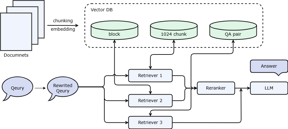
We mentioned the use of QA pairs in Advanced 1 and recommended debugging after learning the vector database. This is because QA pair extraction takes a long time and a lot of tokens. If it is executed every time the system is restarted, it will waste a lot of time and tokens. However, if a persistent storage strategy is used, the waiting time each time the system is restarted can be adjusted. Combined with the document management interface, you can also adjust and delete the QA pairs extracted from large models.
import lazyllm
from lazyllm import bind

# Use Milvus storage backend
chroma_store_conf = {
  'type': 'chroma',
  'kwargs': {
    'dir': 'qa_pair_chromadb',
   },
  'indices': {
    'smart_embedding_index': {
      'backend': 'milvus',
      'kwargs': {
        'uri': "qa_pair/test.db",
        'index_kwargs': {
          'index_type': 'HNSW',
          'metric_type': 'COSINE',
        }
      },
    },
  },
}

rewriter_prompt = "You are a query rewriting assistant, responsible for template switching for user queries.\
Note that you don't need to answer, just rewrite the question to make it easier to search\
Here is a simple example:\
Input: What is RAG? \
Output: What is the definition of RAG? "
rag_prompt = 'You will play the role of an AI Q&A assistant and complete a dialogue task.'\
    ' In this task, you need to provide your answer based on the given context and question.'

# Define embedding model and reordering model
# online_embedding = lazyllm.OnlineEmbeddingModule()
embedding_model = lazyllm.TrainableModule("bge-large-zh-v1.5").start()

# If you want to use the online rearrangement model
# Currently LazyLLM only supports qwen and glm online rearrangement models, please specify the corresponding API key.
# online_rerank = lazyllm.OnlineEmbeddingModule(type="rerank")
# Local reordering model
offline_rerank = lazyllm.TrainableModule('bge-reranker-large').start()

llm = lazyllm.OnlineChatModule(base_url="http://127.0.0.1:36858/v1")

qa_parser = lazyllm.LLMParser(llm, language="zh", task_type="qa")

docs = lazyllm.Document("/path/to/your/document", embed=embedding_model, store_conf=chroma_store_conf)
docs.create_node_group(name='block', transform=(lambda d: d.split('\n')))
docs.create_node_group(name='qapair', transform=qa_parser)

def retrieve_and_rerank():
    with lazyllm.pipeline() as ppl:
        with lazyllm.parallel().sum as ppl.prl:
# CoarseChunk is the default chunk name provided by LazyLLM with a size of 1024
            ppl.prl.retriever1 = lazyllm.Retriever(doc=docs, group_name="CoarseChunk", index="smart_embedding_index", topk=3)
            ppl.prl.retriever2 = lazyllm.Retriever(doc=docs, group_name="block", similarity="bm25_chinese", topk=3)
        ppl.reranker = lazyllm.Reranker("ModuleReranker",
                                         model=offline_rerank,
                                         topk=3) | bind(query=ppl.input)
    return ppl

with lazyllm.pipeline() as ppl:
# llm.share means reusing a large model. If this is set to promptrag_prompt, rewrite_prompt will be overwritten.
    ppl.query_rewriter = llm.share(lazyllm.ChatPrompter(instruction=rewriter_prompt))
    with lazyllm.parallel().sum as ppl.prl:
        ppl.prl.retrieve_rerank = retrieve_and_rerank()
        ppl.prl.qa_retrieve = lazyllm.Retriever(doc=docs, group_name="qapair", index="smart_embedding_index", topk=3)
    ppl.formatter = (
          lambda nodes, query: dict(
              context_str='\n'.join([node.get_content() for node in nodes]),
              query=query)
        ) | bind(query=ppl.input)
    ppl.llm = llm.share(lazyllm.ChatPrompter(instruction=rag_prompt, extra_keys=['context_str']))

lazyllm.WebModule(ppl, port=23491, stream=True).start().wait()
Based on the content of this tutorial on how LazyLLM uses vector databases to achieve persistent storage and high-speed vector retrieval, it can effectively reduce the calculation time of the RAG system in the restart and execution phases, and can also save a lot of token fees from the perspective of certain node groups. Secondly, through the flexible use of the vLLM framework, faster inference speed can be obtained. By using quantified models, hardware requirements can be reduced and hardware costs can be saved while retaining similar generation effects. It can also reduce model loading time when starting the model.