Chapter 11: Performance Optimization Guide: From cold start to responsive acceleration of your RAG

In the previous courses, we learned a variety of strategies and related evaluation methods to improve the effectiveness of the RAG (Retrieval-Augmented Generation) system from both the retrieval and generation perspectives. In order to obtain better retrieval and recall effects, we introduced retrieval through multiple subqueries, multiple node groups, and multiple retrievers, and also introduced a reordering model. Although we successfully improved the recall effect of the system, the introduction of more links and models also increased a lot of calculation and reasoning costs, and the overall execution time of the system increased accordingly. In practical applications, in addition to system effects, we also need to pay attention to the execution efficiency of the system, that is, whether the system can quickly respond to user requests and whether it can quickly implement document and algorithm iterations. This tutorial will take you through a series of related strategies to improve the operating efficiency of the RAG system.

In the process of building the RAG system, in addition to "accurate searches" and "good answers", the execution efficiency of the system is also a topic that needs attention. In the development process of a truly implementation-oriented knowledge base Q&A system, many developers often face a core problem: slow response, poor experience, and no way to start optimization. Ultimately, such problems are often related to performance bottlenecks at each stage of the system.

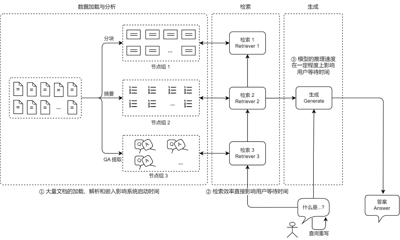
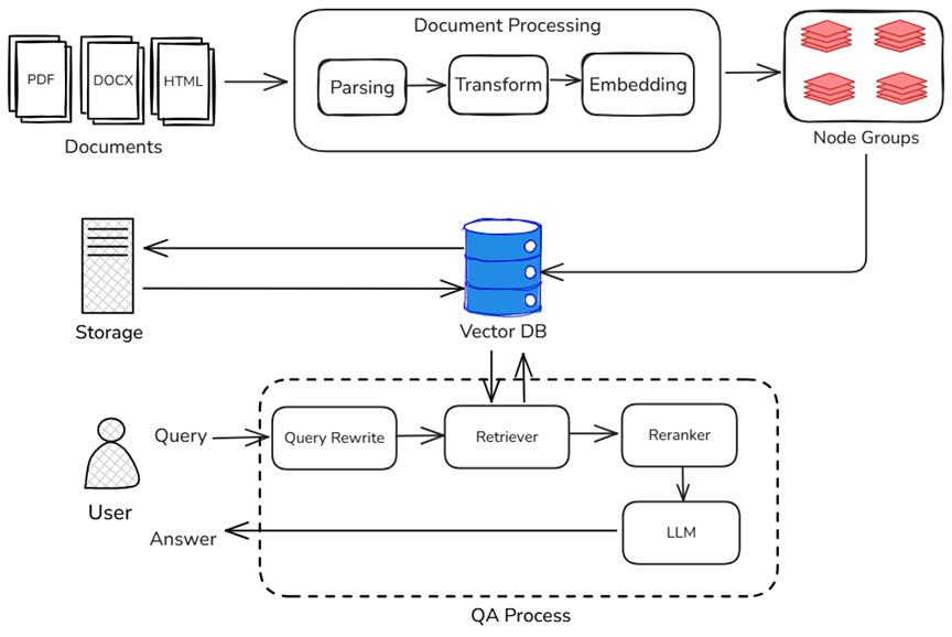
A typical RAG system consists of three major stages: Document storage, retrieval and recall, and generative reasoning. The following figure marks the main factors affecting the overall system performance in each link of the above RAG:

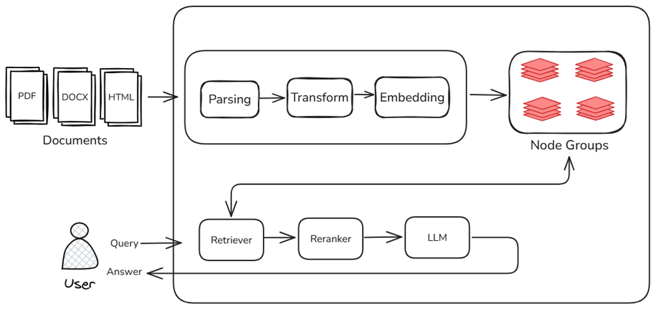
• In the document warehousing stage, the system needs to parse, block, abstract, vectorize and other processes for massive original documents. This stage has a decisive impact on the time-consuming "first startup" or "data update" of the system. The more documents, the slower the startup; the more complex the processing logic, the more memory and computing resources are occupied.
• In the search and recall phase, there are multiple searchers in the system, and the system needs to perform operations such as high-dimensional vector matching, keyword matching, or QA paragraph matching in different node groups. In this process, the retrieval efficiency directly determines the length of user waiting time. If the vector index structure is unreasonable or the retrieval algorithm is not optimized, the overall response speed will be significantly slowed down.
• In the generation inference phase, the recall results are sent to the large model generation module to complete the generation of the final answer. The delay in this stage is mainly related to the inference speed of the large language model itself. But in fact, the delay of the generation module does not exist in isolation, and is also affected by the efficiency of front-end retrieval: slow retrieval → late input → accumulation of reasoning delays, which ultimately affects the overall user experience. Similarly, although streaming output greatly optimizes the user experience during the question and answer process, it can only play a role in the final answering stage in the entire RAG link. Other links that require the participation of large models (such as key information extraction, question rewriting, etc.) will have a greater impact on model inference performance.

p.s. Streaming output can only shorten the first word delay of answer generation, but cannot alleviate the delay caused by using the model in the intermediate stage.

Performance bottleneck analysis of RAG

The operating efficiency of the RAG system is restricted by multiple dimensions. If any link is dropped, it will cause a response bottleneck. This tutorial will provide an in-depth analysis of the performance bottlenecks and optimization strategies in the RAG system from both the hardware and software levels to help developers systematically improve the overall response speed and user experience. The tutorial focuses on the following three topics:

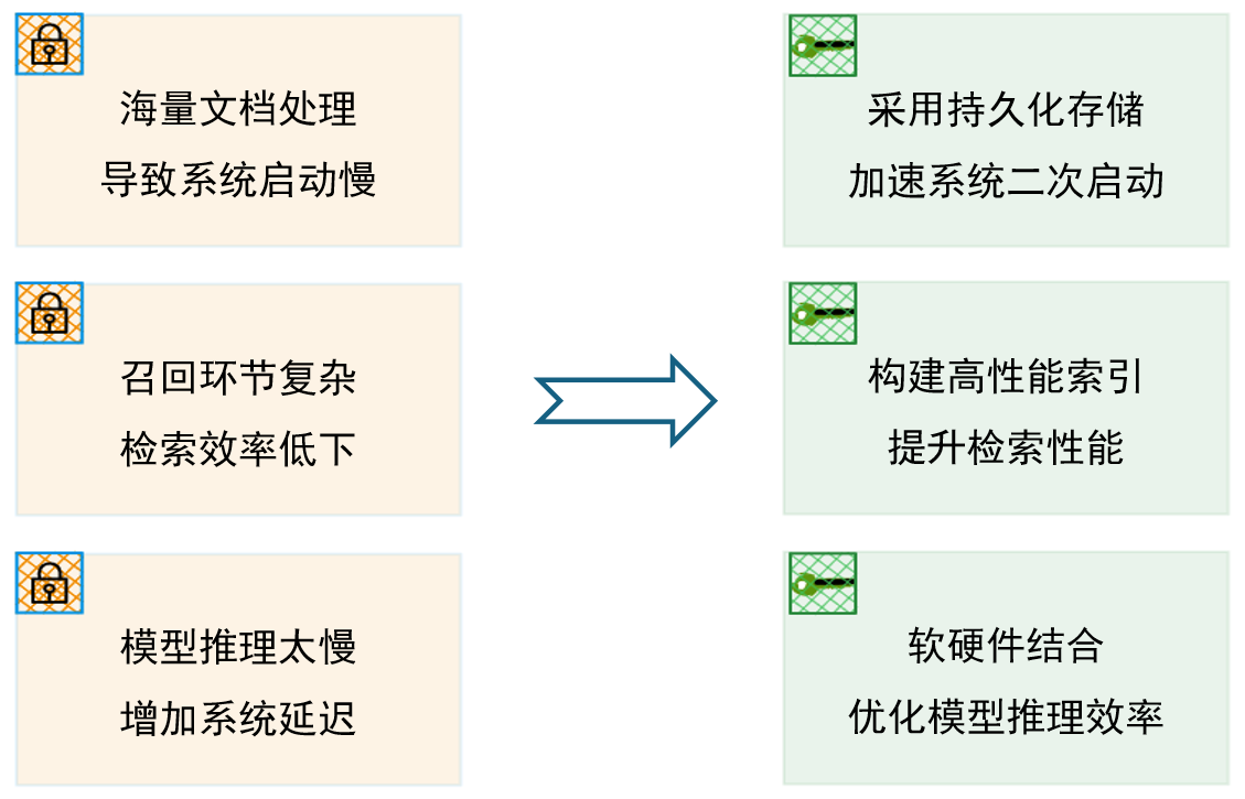
1. Use persistent storage to improve system restart and data loading efficiency Based on the operating principles of computers, the reading and writing characteristics and differences of various storage media are explained, and persistent storage is used to reduce the data loading, parsing and index building time during secondary startup, and provide optimization ideas for system "hot start" and "disaster recovery". At the same time, it introduces the use of caching mechanism to save the performance loss caused by high hit rate data when the system is running.
2. Choose more efficient vector indexes to improve vector retrieval efficiency The system sorts out the data structures, applicable scenarios, and efficient ANN retrieval algorithms of scalar indexes and vector indexes, and compares the performance of mainstream vector databases in terms of construction speed, query performance, memory consumption, etc., to help developers select and implement them, and also introduces the support of LazyLLM in related aspects.
3. Optimize the inference efficiency of large models and reduce delays in the generation phase The system introduces software and hardware-based model acceleration methods and model quantification, model distillation and other technologies to improve the inference speed of the model, thereby accelerating the overall running speed of the system and improving the user experience of the RAG system.

1. Persistent storage

1.1 Computer workflow

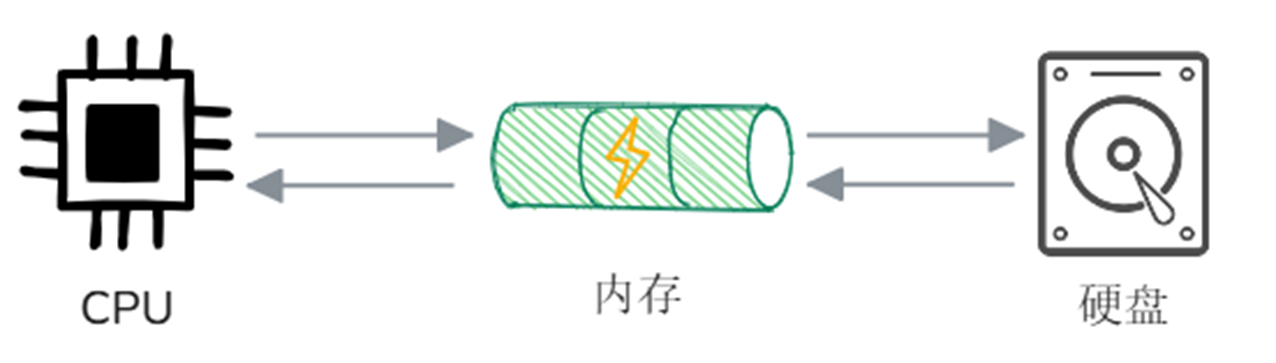
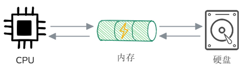
First, let’s review the basic working principles of computers, which mainly involve three core components: CPU, Memory and External storage (such as hard disk). When the computer runs a program, the CPU first notifies the operating system to load the program from the hard disk into the memory. After the program is loaded, the CPU reads the instructions from the memory and starts execution. If a program needs to operate on a file (such as reading or writing), it requests file system access to the hard disk through the operating system. The data will be loaded from the hard disk to the memory, and the program will read or modify the data from the memory. The write operation will first be written to the memory cache, and finally the operating system will write it to the hard disk to ensure that the data is persisted**.

Combined with the above process description, we can try to describe how the previously built RAG system works:

• System startup phase: In this phase, the program will first be loaded from the hard disk into the memory and run after the loading is completed. Then the document storage process will be carried out. In this process, the CPU will request the file system to access the hard disk, load the desired files into the memory, read them, and parse, block, and vectorize them in the memory. After the above process is completed, the vectors and document slices will be temporarily stored in the memory.
• User Q&A phase: The query raised by the user will also be loaded into the memory**. Then the system will execute the retrieval algorithm according to the retrieval type (keyword/vector), find similar document slices in the slice collection temporarily stored in the memory, and combine these slices with prompt words and input them into the large model. Finally, the large model gives an answer based on the input.

If you are careful, you must have discovered that in the running process of the RAG system, except for the document warehousing process during the system startup phase, which involves the "hard disk", the rest of the data processing and storage occur in the "memory". However, storing all data in memory in the RAG system will cause a series of problems:

• Data Loss: Since the memory is "volatile", that is, all the data in the memory will be lost when the power is cut off or the program is restarted (such as sockets, refrigerators, etc.). Therefore, if all data is stored in the memory, once the system is abnormal, data will be lost without backup.

• Slow system startup: Similarly, saving all the data in the memory will cause all documents to be re-entered into the database every time the system is restarted. For scenarios with a large number of documents, it will take a lot of time to complete the document database every time, which is undoubtedly catastrophic to the startup performance of the system.
• High resource usage: During the user question and answer phase, only a very small amount of slice and vector data is needed each time. Storing all data in memory will cause a lot of waste of resources and even affect system performance.

1.2 Use persistent storage to improve system performance

Since storing all data in memory will cause so many problems, should we put it on external storage? The answer is yes. In the RAG system, vector data, slice content and some metadata are usually stored in external storage media (such as hard disks) with the help of vector database to achieve persistent storage and efficient retrieval of data.

Compared with using volatile storage media such as memory, the specific advantages of using persistent storage in the RAG system are as follows:

• Reduce duplicate calculations: Through persistent storage, the system can load stored vector data directly from the hard disk, avoiding the need to re-vectorize all documents every time the RAG system is started, greatly reducing the computational burden at startup;
• Improving memory utilization: Since most vectors are rarely accessed outside the retrieval stage, long-term memory occupation is unnecessary. Through persistent storage, vector data can be released from memory and only relevant vectors are loaded during retrieval, thus improving memory utilization;
• Improve query consistency: If the vector is recalculated every time the system is started, the retrieval results may be inconsistent due to factors such as model updates and random initialization. Through persistent storage in the vector database, the stability of the retrieval results can be ensured and the reliability of the system can be improved.

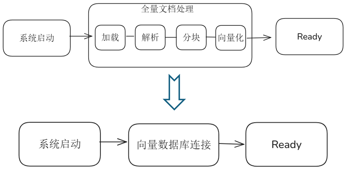
From the above flow chart, you can see the changes in the RAG system startup process after using persistent storage:

• Original: System startup --> Full document loading (document parsing, chunking, vectorization) --> Startup completed
• Now: System startup-->Connect to vector database-->Database connection successful, startup completed

Therefore, the use of persistent storage in the RAG system to save data such as document slices and embedded vectors can reduce the data loading, parsing and index construction time during the second startup of the system, and avoid re-running all data loading processes every time it is started, thereby enhancing the stability of the system and the reusability of data, fundamentally solving the problem of slow startup of the RAG system, and better adapting to complex and changing business needs.

1.3 LazyLLM support for persistent storage

LazyLLM also provides two storage methods based on memory and vector database for developers to choose flexibly. Developers who are in the technology exploration stage can directly use the default construction method in the LazyLLM RAG tutorial. The system will use MapStore by default, and store the slices and vectors after document processing in the memory to achieve the fastest reading and writing speed from document storage to vector retrieval. For RAG systems in the mature stage, LazyLLM provides a variety of vector database support to ensure long-lasting and stable data storage, and significantly shortens the secondary startup time of the RAG system, improving the stability and scalability of the system.

At present, there are many mature vector database solutions, such as open source vector database Chroma, Milvus, etc. In addition, the FAISS library provided by Facebook AI can also be used for efficient vector retrieval and can be used in conjunction with persistent storage systems. Among them, Chroma, which is commonly used in open source vector databases, is suitable for small data storage and rapid prototype development. It provides a simple and easy-to-use API and supports text embedding storage and similarity retrieval. Milvus is suitable for large-scale data scenarios, can support PB-level data storage, supports distributed deployment, and can meet the needs of enterprise-level applications. In addition, Milvus provides a variety of indexing methods to trade off query speed and retrieval accuracy according to different needs.

Among the above-mentioned mainstream vector databases, LazyLLM selected Chroma and Milvus for in-depth adaptation. Whether it is small-scale experiments or enterprise-level application scenarios, it can help developers successfully complete the vector database access required by complex scenarios to help developers achieve a good closed loop from rapid verification in the early stages of the project to stable operation of the project landing.

• Lightweight Experiment: In the early stage of the project, developers can use ChromadbStore in LazyLLM to quickly complete PoC (Proof of Concept) verification, shortening the cycle from idea to runnable prototype.
• Enterprise-level deployment: When the data volume increases or higher requirements are placed on scalability and reliability, Milvus can be smoothly connected to the RAG system using MilvusStore in LazyLLM, making full use of its distributed architecture and multi-index strategy to achieve high concurrency and high throughput vector retrieval services.

Component name	Storage medium	Function description	Applicable scenarios
MapStore	Memory	Memory-based storage provides the basic capabilities of node storage and can realize data reading and writing at the fastest speed	In the technology exploration stage, a small amount of document processing data is stored in the memory to quickly verify technology selection and algorithm iteration
ChromadbStore	Hard disk	Use Chroma vector database to achieve persistent storage of data.	Lightweight experiments, fast POC, shorten the development cycle from idea to runnable prototype
MilvusStore	Hard disk	Use Milvus vector database to realize local storage/distributed remote storage of data.	Enterprise-level deployment, suitable for scenarios with large data volumes and high requirements for concurrency and retrieval performance

Persistent storage improves startup efficiency - LazyLLM

documents = lazyllm.Document(dataset_path="xxx", embed=xxx, …, store_conf={…})

1.4 Extended learning (optional)

​ Program running mainly involves three core components: CPU, memory and external storage (such as hard disk).

• The program is loaded from the hard disk into the memory and run
• The CPU reads program instructions from memory and executes them
• Data reading: The CPU requests the operating system to access the hard disk, and the data is loaded from the hard disk to the memory.
• Data writing: The CPU first writes the data to the memory, and finally the operating system writes the data to the hard disk to achieve persistent storage.

1.4.1 Memory and hard disk

Memory (usually referred to as RAM) and hard disk (Storage (usually referred to as SSD/HDD)) are the two main storage media in computers, each with different roles and functions.

Memory is a temporary storage device in a computer, mainly used for data exchange between the CPU and the hard disk. It is a temporary working space when the computer executes programs and processes data. Memory has the following characteristics:

• High-speed access: The memory has extremely fast read and write speeds, usually measured in nanoseconds (ns), and the CPU can quickly access and process the data in the memory.
• Volatile: All data in the memory will be lost when the computer is powered off or restarted, so it is called "volatile storage".
• Relatively Small Capacity: Currently, common computer memory capacities generally range from a few GB to several hundred GB.
• Random access capability: The CPU can access data at any location in the memory in any order and at the same speed.

Hard drive is a computer's persistent storage device, used for long-term storage of programs, data, and files. Even if the computer is shut down, the data on the hard drive will not be lost. Hard drives usually have the following characteristics:

• Persistent Storage: Once the data is written to the hard disk, it will not be lost even if the power is cut off, and the data can be saved for a long time.
• Large Capacity: Compared with memory, hard disks have larger storage capacity, usually from hundreds of GB to several TB or even tens of TB.
• Slower access speed: Traditional mechanical hard disks (HDD) usually have millisecond delays when accessing data, while solid state drives (SSD) are much faster, but the overall speed is still much lower than memory.
• Data access method:
  • Mechanical hard disk (HDD): Data access is completed through head seeking and turntable rotation, and there is a seek delay.
  • Solid State Drive (SSD): Using flash memory technology, no mechanical parts, faster access, more stable and reliable.

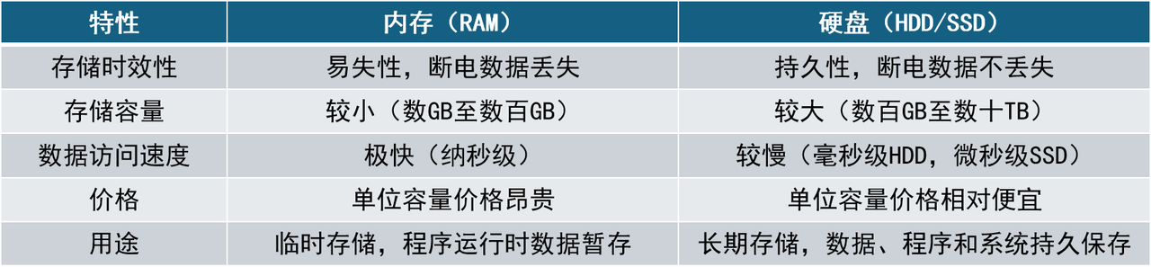
Features	Memory (RAM)	Hard drive (HDD/SSD)
Storage timeliness	Volatility, data is lost when power is turned off	Durability, data is not lost when power is turned off
Storage capacity	Small (several GB to hundreds of GB)	Large (hundreds of GB to tens of TB)
Data access speed	Extremely fast (nanosecond level)	Slow (millisecond level HDD, microsecond level SSD)
Price	The price per unit capacity is expensive	The price per unit capacity is relatively cheap
Purpose	Temporary storage, temporary storage of data when the program is running	Long-term storage, persistent storage of data, programs and systems

Table: Differences in memory and hard disk characteristics

There are significant differences in speed and characteristics between memory and hard drives. In terms of access speed, the read and write latency of memory is measured in nanoseconds, while the seek delay of mechanical hard disks is usually measured in milliseconds. The memory access speed is about 100,000 times faster than mechanical hard disks and about 1,500 times faster than SSDs. This means that obtaining data from memory is almost instant, while reading from hard disks may take several milliseconds or even longer. The extremely fast access capability makes memory-based document storage and information retrieval the first choice for applications with high real-time requirements. However, although memory is fast, it is a volatile resource, and data will be lost after a power outage or restart. In contrast, hard drives (such as SSD) have data persistence and capacity advantages, and are more suitable as long-term storage media.

Although there is a huge difference in speed between hard disks and memory, in recent years, hard disk technology has continuously improved from traditional mechanical hard disks (HDD) to SATA interface solid state drives (SSD) to high-speed NVMe SSDs, mainly reflected in random access latency and data throughput. HDD uses mechanical rotating disks and magnetic heads for seeking, and the average addressing delay is at the millisecond level (a typical 7200-rpm HDD delay is 4.17ms); while SSD has no mechanical parts and relies on electronic storage units. The read and write delay of SATA SSD can be as low as tens of microseconds (such as Intel enterprise-class SATA SSD delay of 0.036ms), and the delay of NVMe SSD (especially Optane class storage using high-speed bus) can even reach 5µs (0.005ms). In addition, the I/O throughput capabilities of different media vary greatly: HDDs can only process a few hundred random I/O operations per second (IOPS), while SATA SSDs can handle tens of thousands of operations, and NVMe SSDs can easily handle millions of operations. The following table compares typical performance metrics for these storage media:

Storage media	Average latency (Random Latency)	Random IOPS	Sequential throughput (Seq. Read)
HDD (7200 rpm)	4.2 ms	400	150 MB/s
SATA SSD	0.036 ms	97,000	600 MB/s
NVMe SSD	0.005 ms	1,500,000	7200 MB/s

As shown above, SSD, especially NVMe SSD, has an order of magnitude improvement in random read and write performance compared to HDD. Even in sequential read and write scenarios, NVMe SSD can achieve a throughput of several GB per second, which is dozens of times that of mechanical hard disks. This means that if large-scale text slices and vector data are stored in SSD, I/O bottlenecks can be significantly reduced and the overall response speed of the RAG system can be improved. Of course, this improvement comes at the cost of higher costs, so there needs to be a trade-off between capacity, performance and cost in actual deployment.

Extremely fast access capabilities make memory-based document warehousing and information retrieval the first choice for applications that require high real-time performance. This is also the reason why we loaded all data into memory in the previous tutorial. In the early stages of development of the RAG system, because technology selection (such as Embedding model, Reader) and system design (such as blocking strategy, node group design) have not yet been determined, there are frequent technical iterations during the research and development process. Compared with the stable storage of massive document processing data, developers are often more inclined to select a small number of typical documents and combine advanced algorithms and engineering optimization technologies to verify the actual performance of the system. Therefore, temporarily storing data such as text slicing and vector embedding in memory for retrieval can obtain query responses as quickly as possible.

However, as the memory characteristics are introduced above, it is "volatile". Once the service process is restarted or the machine crashes, the document slices and vector indexes previously saved in the memory will disappear, and the next time you run the program, you will have to "start all over again." Therefore, memory storage is only suitable for accelerated development and small-scale experiments. As the system design and algorithm optimization gradually become stable, a large number of formal documents need to be stored in the database for retrieval. At this stage, no one wants to spend a lot of time waiting for documents to be re-entered into the database every time the program is run, so we usually need to save these data to the hard disk.

1.4.2 Memory cache mechanism: pre-store high-heat data to accelerate system response

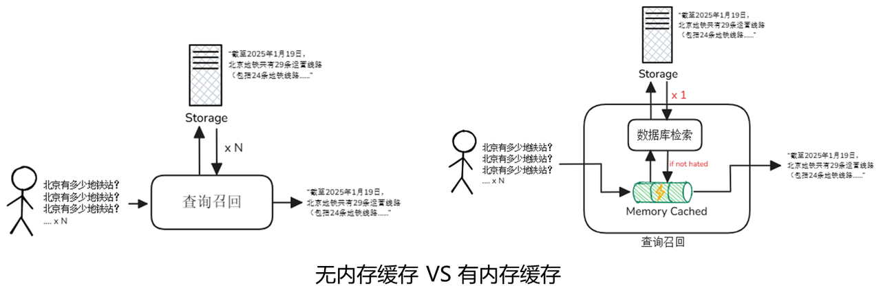
For a high-performance system, the choice between memory and hard disk is never OR, but AND. In view of the disadvantage that disk is slower than memory, a cache layer is often introduced in actual system architecture to use memory cache to make up for the difference in disk speed. The Memory Cache mechanism is an optimization strategy that reduces repeated calculations and external retrieval by pre-storing frequently accessed data. Proper use of the cache mechanism can significantly improve system response speed and reduce resource consumption.

In RAG scenarios, "hot" data, such as frequently queried vectors or retrieval results, are usually cached in memory, so that subsequent similar queries can obtain these data directly from memory, thereby reducing repeated calculations and disk I/O, thereby making up for the performance gap of disk storage to the greatest extent, allowing RAG retrieval to take into account persistence without losing speed. We assume that in a retrieval system, users frequently ask "How many subway stations are there in Beijing?". During the first processing, when the system requests database retrieval, the database will read the relevant embedded vectors and slice data from the hard disk and answer the question, which takes a long time. Then the system will cache the results. The next time this question is asked, the relevant content will be returned directly from the memory, which greatly improves the system's response speed.

In modern computing systems, the memory cache mechanism is an optimization strategy that reduces repeated calculations by pre-storing frequently accessed data. By "exchanging memory for time", it significantly improves system response speed while reducing the consumption of underlying storage and computing resources. The implementation of memory caching mechanisms usually relies on high-performance memory caching systems, of which the two most commonly used solutions are Redis and Memcached. They each have their own characteristics and are suitable for different application scenarios.

Redis is one of the most widely used in-memory caching systems today. It not only supports simple key-value caching, but also has built-in rich data structures, such as List, Set, Zset, Hash, etc., which can meet the caching needs of various structured and semi-structured data. The following are the core features and typical application scenarios of Redis:

Core features:

Multiple data structure support: Redis provides multiple data structures to facilitate processing of complex data relationships.

TTL (expiration time): Supports flexible setting of cache life cycle, and automatically cleans expired data through TTL.

Persistence mechanism: Supports two persistence methods: RDB (snapshot) and AOF (log append), which can restore data even after memory loss.

Lua script: Built-in Lua script support, suitable for implementing complex atomic operations.

Typical usage:

Hot vector cache: In the RAG (Retrieval-Augmented Generation) system, Redis can be used to cache frequently accessed vectorized data to reduce retrieval calculation overhead.

Session context management: In the dialogue system, Redis can cache the user's session history and provide context correlation capabilities.

Ranking: With the help of ordered sets (Zset), Redis can easily implement the ranking function.

Compared with Redis, Memcached is a more lightweight memory caching solution that focuses on "high-speed key-value reading and writing". It is known for its minimalist design and high performance, and is suitable for caching data with a short life cycle, high access frequency but simple structure.

Core features:

Pure memory storage: Memcached does not support persistence. Data is completely stored in memory and will be lost when power is turned off.

Simple protocol: Supports simple and efficient text protocols, reducing communication overhead.

Ultra-low latency: Read and write latency can reach microsecond level, suitable for scenarios that require extreme performance.

Typical usage:

Model parameter caching: In machine learning or deep learning systems, Memcached can be used to cache frequently used model parameters to reduce computing costs.

Session cache: used to store users’ temporary session information and supports high concurrent access.

HTML fragment caching: In web applications, Memcached can cache dynamically rendered HTML fragments to improve page loading speed.

Although Redis and Memcached have functional differences, they both effectively improve data access speed by "exchanging memory for time". In the RAG system, the reasonable introduction of the memory caching mechanism can not only improve the performance of a single query, but also significantly reduce the pressure on the underlying database, making the entire question and answer process lighter and more efficient while ensuring accuracy.

1.4.3 Scalar database and vector database

For data such as documents, slices, and vectors stored in the hard disk, the system usually uses a database to perform add, delete, modify, and query operations. Database is a software system used to store, manage, retrieve and operate data in an organized manner. It has the characteristics of efficient storage, efficient access, and support for concurrency and consistency. According to the type of data stored, databases can be divided into scalar database and vector database.

Scalar databases are the traditional databases we come into contact with most every day, such as MySQL, PostgreSQL, MongoDB, etc. They mainly process structured data, that is, table-like information with clear fields, such as the user's name, gender, date of birth, order time, price, status, etc. Scalar databases are good at precise queries, aggregate analysis, transaction processing and other tasks, and are widely used in finance, auditing, medical care, supply chain and other fields. Take PostgreSQL as an example. It supports complex SQL statements, full-text search, JSON structure, and can also perform spatial queries with geographical information. It is very suitable for building business systems for medium and large enterprises.

Vector database is a new type of database that has been widely used with the rise of AI. It is mainly oriented to feature vector storage and similarity retrieval tasks of unstructured data, such as text vectors, image vectors, etc. These data are usually high-dimensional floating-point arrays encoded through large models, and traditional databases are not good at managing this type of data. Vector databases specifically provide efficient vector index structures (such as HNSW, IVF, PQ), which can efficiently retrieve large-scale data (the content of vector indexes will be introduced in the next section). At the same time, some vector databases also support hybrid filtering of vectors + metadata to facilitate retrieval, recommendation and multi-modal question and answer based on semantic understanding.

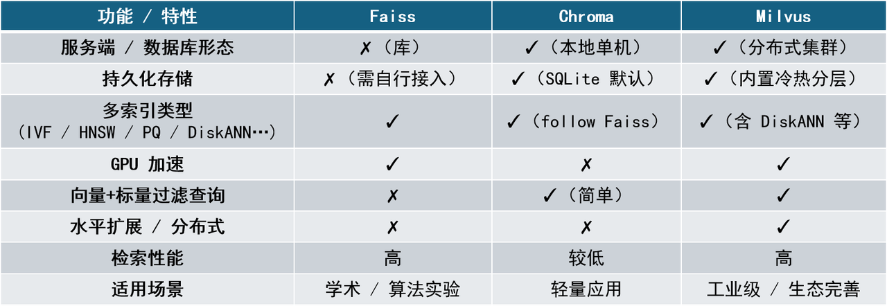
Currently, the more mainstream vector databases include Chroma, Faiss, and Milvus. These systems have their own characteristics in terms of retrieval performance, deployment complexity, functional richness and ecological support, and are suitable for different business scenarios. Their positioning and characteristics will be introduced one by one below.

• Faiss
  • Faiss is a high-performance vector search library open sourced by Facebook AI. Its core advantage lies in its extremely optimized C++ implementation and powerful indexing support. Faiss is not a database, but a "tool library" that provides the implementation of a series of vector indexing algorithms, including Flat, IVF, PQ, HNSW, etc. Faiss is positioned at the lower level and is usually used to build custom vector systems. It is suitable for teams or developers who have the ability to encapsulate services, manage storage and persistence on their own.
• Chroma
  • Chroma is a vector database positioned as lightweight, localized, and quick to deploy, focusing on "out-of-the-box" user experience. It tightly binds "document + metadata + embedding vector", uses SQLite storage and FAISS as the index engine by default, and supports simple filtering and data separation by namespace. Chroma is suitable for the rapid development of small projects or prototype systems, and is especially suitable for individual developers, local testing, and education scenarios. However, it still has obvious shortcomings in distributed deployment, index type flexibility, large-scale retrieval optimization, etc.
• Milvus
  • Milvus is a full-featured vector database developed by Zilliz with the goal of building an "industrial-grade vector retrieval system". It has complete vector life cycle management capabilities, supports millions or even billions of vector storage and retrieval, and is suitable for deployment in production environments such as clouds and server clusters. Milvus's architecture supports distributed deployment, hot and cold tiered storage, vector + scalar mixed filtering queries, and provides SDK and RESTful/gRPC interfaces.

Name	Main features	Advantages and disadvantages	Applicable scenarios
Faiss	Supports multiple efficient vector indexing algorithms (including GPU-accelerated versions). Accuracy and speed can be flexibly traded off through configuration. Provides Python/C++ interface	Advantages: Extremely high performance, suitable for large-scale vector searches. Supports index compression and GPU acceleration. Fully customizable control of storage structure and index update logic. Disadvantages: Does not include server-side functions, no native persistence, and metadata management capabilities. Deployment requires additional packaging or access to external components (such as SQLite, Redis)	Embedded scenarios, customized search systems, model evaluation or research projects
Chroma	Built-in embedded generation module (supports OpenAI, Instructor, etc.), friendly for local deployment, supports Python calls and REST API, supports vector retrieval and metadata filtering, does not support complex index structures, and query efficiency is limited by the default configuration of FAISS	Advantages: No need to rely on back-end services, extremely simple deployment, integrated with a variety of large model application development framework tools, active community, fast development iteration Disadvantages: Average query efficiency, limited indexing capabilities, does not support distribution, not suitable for large-scale vector storage and high concurrency scenarios	Small applications, local document Q&A, educational demonstrations, RAG introductory experiments
Milvus	Multiple ANN indexes (HNSW, IVF, DISKANN) metadata filtering, Boolean filtering, multi-field combined queries support distributed, horizontal expansion, hot and cold separation storage interfaces are rich, support calling Python, Java, Go, etc.	Advantages: Functionality: Not only supports basic vector similarity search, but also supports advanced functions such as sparse vectors, batch vectors, filtered search and hybrid search functions. Flexibility: Supports multiple deployment models and multiple SDKs, all within a powerful integrated ecosystem. Performance: Using optimized indexing algorithms such as HNSW and DiskANN and advanced GPU acceleration to ensure high throughput and low-latency real-time processing. Scalability: Its custom distributed architecture scales easily from small datasets to Collections of over 10 billion vectors. Disadvantages: Complex architecture, high deployment threshold, may require more tuning and configuration	Enterprise-level document search, image search, recommendation system, RAG service deployment

2. Efficient index construction and vector retrieval algorithm

2.1 Index

2.1.1 Introduction to index

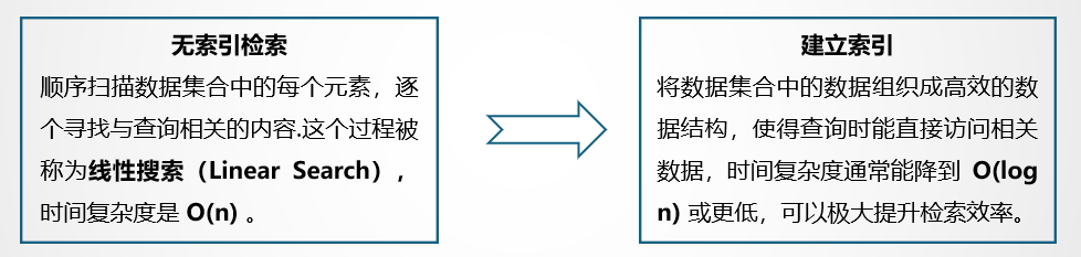
Index is a special data structure whose function is to pre-organize the structure of the data so that the searcher can efficiently locate and retrieve relevant information. Simply put, an index is like a table of contents in a book that helps locate specific information quickly without having to search page by page. Just imagine that if there is no index, the searcher must sequentially scan each page of the book to find content related to the query word by word. This process is called Linear Search (Linear Search). The time complexity of linear search is O(n), where n is the number of documents or the total number of words in the document. As the amount of data increases, linear search becomes extremely inefficient. By building an index, the information in the document can be organized into an efficient data structure, so that relevant data can be directly accessed during query. The time complexity can usually be reduced to O(log n) or lower, which can greatly improve the retrieval efficiency.

The figure below takes a dictionary as an example to show the impact of indexing on the search process. Suppose there is a dictionary with N words starting with each letter, then the dictionary has a total of 26*N words. Our goal is to find the word "retrieve" from the dictionary. The left side of the figure shows the linear search method, starting with words starting with a and searching one by one. r is the 18th letter in the alphabet. Finding the word "retrieve" requires (17N+i) queries, (assuming "retireve" is the i-th word starting with r words); the right side of the picture shows the search method using the dictionary tree index, which only requires (18+5+20+18+9+5+22+5=102) times, where 18 is the serial number of r among the 26 letters, 5 is the serial number of e, and so on. If N=100, the number of queries between the two is (1700+i) vs 102, 1<=i<=100. The larger N is, the larger the difference in calculation amount is. It is clearly visible which calculation efficiency is higher or lower.

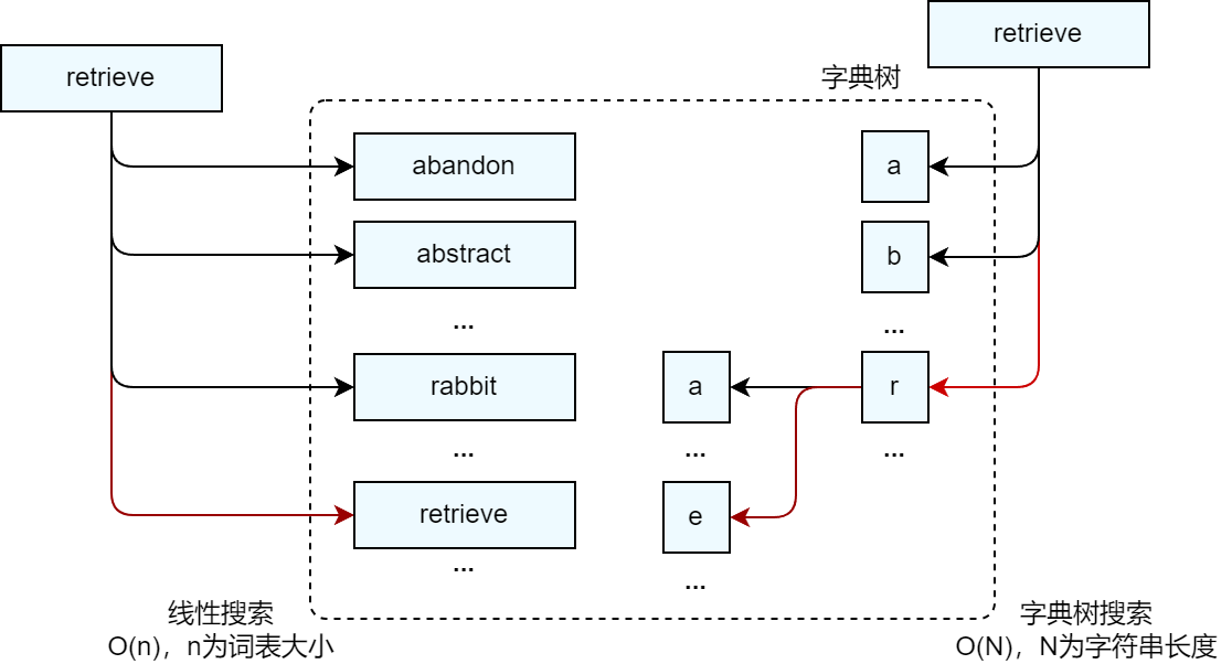
In fact, when using the dictionary tree to query any word, you only need to perform at most (26m) queries, where m is the length of the queried word, which means that the query complexity can be reduced to O(m)*. Through the above examples, we can feel that using indexes can significantly reduce the number of calculations during the retrieval process and improve retrieval efficiency.

scalar index:

Scalar index is a data structure established for scalar column values ​​(such as numbers, strings, Boolean values, dates, etc.) in traditional relational databases to help the database find data efficiently.

Scalar indexes have the following four main functions:

• Significantly improve query speed: Help the database directly locate the target location in the data file, thus effectively avoiding the time-consuming operation of full table scanning.

• Reduce the number of disk I/O: The database does not need to read the entire data set, which greatly reduces the burden of disk I/O.

• Optimize sorting and grouping operations: enable the server to avoid sorting and using temporary tables, thereby improving query efficiency.

• Improve the performance of complex queries: It can provide efficient support for complex query operations, such as when performing table join operations, or when searching for maximum values, minimum values, etc.

Vector Index:

Vector index is an index structure used to accelerate similarity retrieval of high-dimensional vector data. Its goal is to quickly find several vectors that are most similar (Top-K) to a certain query vector in large-scale data sets.

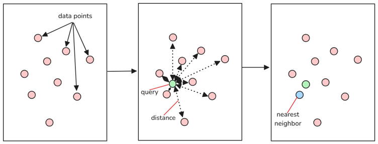
Vector retrieval in the RAG system can be described as "given a query vector q, find several vectors with the smallest (or largest) distance (or similarity) in the vector set V." This process is called nearest neighbor search (Nearest Neighbor, NN). When Top K exists in the search parameters, that is, when the top K data items that are most similar to the target data need to be found, the above search process evolves into K-Nearest Neighbor (K-NN).

The problem is exposed: the vector size becomes larger and the amount of calculation increases dramatically.

2.1.2 Index in LazyLLM

In previous courses, we learned that the recall effect of the RAG system can be effectively improved by combining multiple node groups with different similarity calculation methods. Similarly, LazyLLM has built-in default index DefautIndex and vector index SmartEmbeddingIndex, and provides an index component (IndexBase) to support custom index design. You only need to simply define three functions (update to insert nodes, remove to delete nodes, and query to query nodes) to quickly implement flexible indexing.

From the perspective of framework design, LazyLLM has clear levels of components and clear division of labor. It is more readable and scalable than other mainstream application development frameworks. The following is an overview of the Index component in Llamaindex, another mainstream application development framework.

The base class of the index component in Llamaindex is IndexBase, which defines dozens of input parameters and methods for other subclasses to implement various complex functions. In the index definition of Llamaindex, after it receives a set of nodes, it cannot be queried directly. Instead, it needs to be combined with the built-in methods as_retriever, as_query_engine, etc. to convert the Index into a retriever or query engine, and then call the corresponding query method in the retriever or query engine for retrieval. This design makes developers feel strange when reading the source code - it is obviously an index, but after entering the node collection, it cannot be directly used to retrieve it. Instead, there are many built-in "detours" to turn around. At the same time, although it has many built-in "Index types", many of them are not in the "index" category, and the concept is quite confusing. The following is a table presentation of some typical indexes sorted into the conceptual framework of LazyLLM.

Index type	description	node group	similarity	index
SummaryIndex	A simple data structure that stores documents as a sequence of nodes. During index building, document text is chunked, converted into nodes, and stored in a list. Used to retrieve documents containing specific keywords or phrases.
VectorStoreIndex	Vector index, during the storage process, the embedding model will be called to vectorize the text	X	cosine	vector index
DocumentSummaryIndex	Extract and index document summaries using large models	summary	llm/cosine	X
KeywordTableIndex	Use a large model to extract keywords from document fragments and build a keyword index	X	llm extraction	linear

It can be seen that some typical Indexes do not have a single clear concept, but implement many functions with mixed concepts through various configuration parameters. In contrast, in the definition of LazyLLM, the file is divided into node groups (Transform) according to rules and indexed (Index), and then a retriever (Retriever) is used to obtain the data set most similar to the target data based on a specific similarity type (similarity). This process and definition appear to be extremely refreshing.

2.2 Efficient vector database

For developers, writing a vector indexing algorithm from scratch to achieve efficient retrieval is definitely not what we want. Vector indexing is precisely one of the core capabilities of vector databases. We can simply think of it as:

Vector Database = Vector Index + Vector Storage + API Support + Metadata Management

Efficient indexing algorithms are integrated into major vector databases. After the system writes vectors to the database, the vector database can use vector indexes to quickly locate the most similar vectors during query, greatly improving response speed.

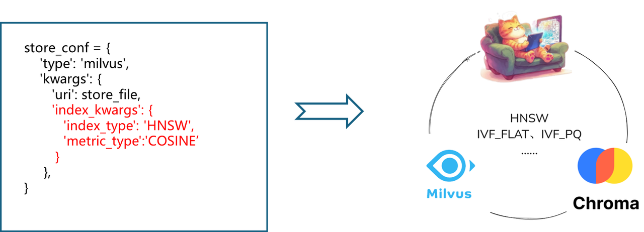
In the design of LazyLLM, flexible configuration of the vector database can be achieved through the store_conf parameter of Document, where the 'type' field specifies the specific database type. When we use LazyLLM to build a RAG system, we only need to specify the storage configuration item store_conf in the Document, and write the corresponding vector database type and database-related configuration (such as local storage path, index type used, etc.) in it to achieve access to the vector database. In addition, for the Milvus vector database, LazyLLM natively supports its unique scalar index function. The filter field is passed in during the retrieval process. No manual filtering is required, and nodes are filtered according to the scalar index to achieve complex retrieval of vectors + scalars.

2.3 Engineering optimization: the “invisible pusher” for performance improvement

When discussing performance optimization of RAG systems, we tend to focus on algorithm optimization and technology selection, such as using more efficient index structures, better recall strategies, more appropriate vector databases, etc. However, it is not just the algorithm and database itself that affects the performance of the RAG system. Optimization at the engineering level is often the key to determining whether the system can be implemented stably and efficiently.

In engineering, we usually divide tasks into two broad categories:

• IO-intensive tasks: The main bottleneck lies in input/output operations such as disk reading and writing, network transmission, and database access. The processing speed of such tasks is limited by the response time of external devices. Typical scenarios: file transfer, calling remote API, etc.
• Computing-intensive tasks: The main bottleneck lies in its own calculation volume, which relies on the CPU or GPU to perform a large number of mathematical calculations. Typical scenarios: local model inference, data analysis, etc.

Parallelism and Concurrency

Parallel Processing is a computing method in a computer system that can execute two or more processes simultaneously. Can work on different aspects of the same program at the same time. The main purpose is to save time in solving large and complex problems.

Concurrency Processing: Refers to a period of time in which several programs are running between startup and completion, and these programs are all running on the same CPU, but only one program is running on the CPU at any point in time.

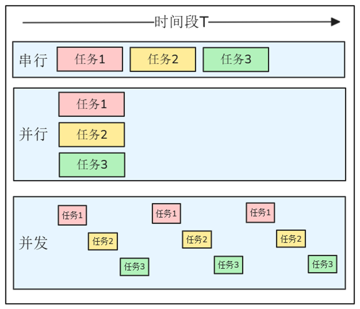
• In life: Chef in a restaurant
  • Serial: A chef first washes vegetables → then stir-fries → then boils soup → finally steams rice
  • Parallel: three chefs are responsible for stir-frying, boiling soup, and steaming rice → at the same time without affecting each other
  • Concurrency: A chef has multiple stoves. He puts the dishes down and waits for 3 minutes. During these 3 minutes, he will stew the soup. During this period, he will come back to stir-fry, season, and plate.
• In the program: document parsing
  • Serial: Massive documents are parsed one by one
  • Parallel: open multiple threads and parse multiple documents at the same time
  • Concurrency: In the same thread, let the file I/O waiting time be "vacated" for other tasks. During this period, do not be idle and do other things.

Parallelism in Python

Parallelism in Python is mainly implemented using multi-processes and multi-threads.

• Multi-threading (Thread): execute multiple threads concurrently within the same process; share the memory and resources of the process.
  • Core features:
    • Thread switching overhead is small and fast startup
    • Constrained by CPython GIL, only suitable for I/O intensive
    • Data sharing is simple, but race conditions are prone to occur; synchronization methods such as locks and queues are required
  • Python implementation: ThreadPoolExecutor thread pool in concurrent.futures
• Multi-process (Process): The same program replicates multiple independent processes at the operating system level; each process has an independent memory space and Python interpreter.
  • Core features:
    • True multi-core parallelism, not restricted by GIL
    • Inter-process communication requires IPC (queue, pipe, shared memory)
    • High creation and switching costs, slow process startup
  • Python implementation: using multiprocessing to implement multiple processes

GIL (Global Interpreter Lock)

Global Interpreter Lock (GIL, Global Interpreter Lock) is a global mutex lock that prevents multiple threads of the interpreter from concurrently executing machine code. Its core function is to ensure that only one thread executes Python bytecode at the same time.

The inevitability of GIL’s existence is caused by the following circumstances:

• Issues left over from history: Python’s early design adopted a reference counting memory management mechanism, which did not consider the concurrency requirements of the multi-core era.
• Thread safety guarantee: Prevent multiple threads from modifying object reference counts at the same time causing memory leaks (such as two threads releasing the same object at the same time)
• Ecological dependencies: A large number of Python extension libraries are developed based on the thread safety assumption of GIL, and the cost of removal is extremely high

Technical solutions to bypass the GIL:

• Multi-process parallelism (multiprocessing, using Queue, Value, and Array to flexibly realize memory sharing between processes)
• Asynchronous programming model (asyncio achieves single-threaded high concurrency and is suitable for I/O-intensive scenarios)
• Hybrid programming extension (implement core algorithms in C/C++, such as NumPy, Pandas and other scientific computing libraries)

Note: The function of asyncio is to schedule the execution of the code of each task through a python object called event loop. When a task is executed, other tasks will not take their turn to execute until the task actively returns control. (This is significantly different from threading concurrency). Because the code needs to be designed to implement the subtasks and the controller before the main program, "asynchronous" code is more complex and troublesome than threading concurrency and multiprocessing.

Value of thread

In engineering, we usually divide tasks into two broad categories:

• Compute-intensive (CPU-intensive) tasks:

  • Refers to tasks that mainly involve a large amount of calculation and processing during the execution process, such as performing complex calculations, algorithms or logical operations, but involving relatively few IO operations.
  • Typical scenarios: Local model inference, data analysis, etc.

• IO intensive tasks:

  • Refers to tasks that usually require interaction with external resources during execution, most of the time is spent waiting for input and output (IO) operations to be completed, and the actual calculation amount is relatively small.
  • Typical scenarios: reading and writing files, network requests, database queries, etc.

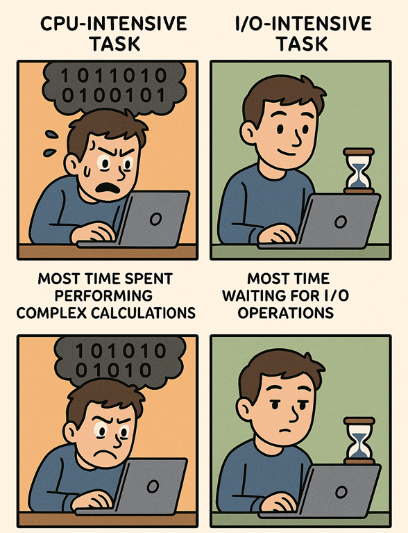
Python's multithreading is designed for IO-intensive tasks!

Performance optimization of RAG in LazyLLM

In the RAG system, IO-intensive tasks and computing-intensive tasks widely exist and are executed interleaved. If not optimized, resource congestion, processing delays, and even system-level performance bottlenecks can easily occur. For RAG scenarios, LazyLLM has made a lot of efforts in engineering optimization:

• Multi-threading & asynchronous scheduling: LazyLLM natively supports multi-threading and asynchronous mechanisms. For IO-intensive tasks, using the ThreadPoolExecutor provided by LazyLLM can make full use of the idle time during waiting for network transmission and greatly improve resource utilization. At the same time, LazyLLM's Flow component provides parallel components Parallel, Warp, and Diverter. These components can make full use of system resources and realize parallel computing of data.
• Batch processing mechanism: In the RAG system, the document slicing vectorization process is computationally intensive and time-consuming. To address this problem, LazyLLM adopts a batch processing mechanism, which greatly reduces the time-consuming vectorization process by vectorizing a batch of slices at the same time. At the same time, for massive document parsing scenarios, LazyLLM provides a multi-process mechanism to complete document parsing in batches. The above-mentioned batch processing mechanism greatly improves the speed of the RAG system in the document warehousing process.

The improvement of RAG system performance not only depends on the vector index you use and which vector database you choose. Deeper optimization often comes from whether you have done enough work in engineering implementation. The algorithm determines the upper limit, and engineering determines the lower limit. Both are indispensable.

2.4 Extended learning

2.4.1 Classification of indexes

According to the type of data storage, indexes can be divided into two types: scalar index and vector index.

scalar index

Scalar indexes are indexes established for scalar values (such as numbers, strings, Boolean values, dates, etc.) in traditional relational databases to help the database obtain data efficiently. Taking the MySQL database as an example, the index of the MySQL database can be regarded as a sorted list of values ​​in a column or multiple columns in the database table. Through this list, the database system can quickly find data records with compound conditions without scanning the entire data table row by row. For the MySQL database, indexes mainly have the following four functions:

• Significantly improves query speed: Indexes can significantly improve query speed, especially when the amount of data is large. Without an index, MySQL would have to read the entire table row by row until the target row is found. But with the index, MySQL can directly locate the target location in the data file, thus effectively avoiding the time-consuming operation of full table scan.
• Reduce the number of disk I/O: Indexes can reduce the number of disk I/O required to obtain a record in the table. With the help of indexes, MySQL can quickly locate the corresponding location in the data file without reading the entire data set, which greatly reduces the burden of disk I/O.
• Optimized sorting and grouping operations: Indexes help the server avoid sorting and using temporary tables, thereby improving query efficiency. When processing queries related to sorting and grouping, indexes can exert their unique advantages and optimize the query execution process.
• Improve the performance of complex queries: Indexes can provide support for complex query operations, such as when performing table join operations, or searching for maximum values, minimum values, etc. The existence of indexes allows these complex queries to be executed more efficiently. The main data structures used in scalar indexes include B+ trees, hash tables, jump tables, etc.

Commonly used scalar index structures include supplementary B-tree/B+ tree, hash table and skip table.

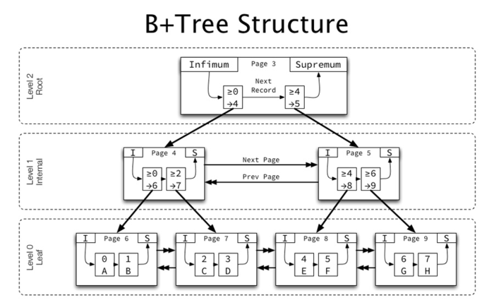
B tree / B+ tree

As the most popular database index data structure, B-tree/B+ tree is a multi-fork balanced search tree. The original design is to allow one disk I/O to read the entire node data, thereby maximizing sequential reading and minimizing random addressing; B+ tree is its most common variant. The difference is that all data records are only stored in leaf nodes, and internal nodes only store key values ​​and point to child nodes, forming an ordered linked list between leaves, and range scanning is particularly efficient.

characteristic:

• Logarithmic level query, insertion, deletion - all paths are of equal length and the complexity is \(O(log \text{mN})\).
• Disk Affinity - Node size is usually consistent with disk pages, reducing I/O times.
• Natural support for range queries - Sequential traversal of leaf linked lists can quickly obtain interval results.

Compared with balanced binary trees, B-trees have improved node space utilization. Each borrowing point stores more data, reduces the height of the tree, and improves query performance.

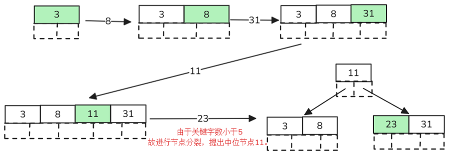
B-tree construction:

Define a 5-order tree and insert data 3, 8, 31, 11, 23...

• Node splitting rule: m=5, the number of keywords must be less than or equal to 5-1=4
• Sorting rules: node comparison - small on the left and large on the right

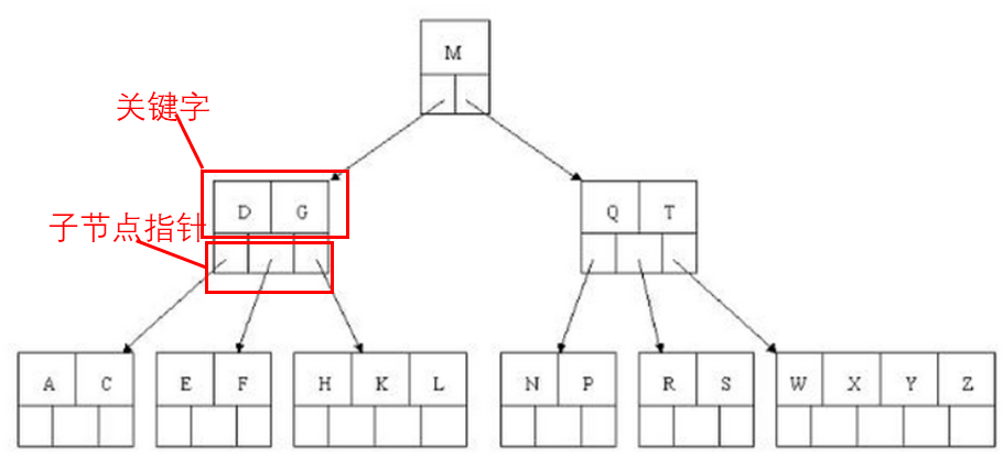
Find the letter "E":

1. Get the root node comparison. According to the dichotomy method, the left is small and the right is large, E<M, so go to the left child node to query;
2. Get the keywords D and G. Since D<E<G, we go to the middle child node to query;
3. Get E, F, E=E, so the keyword and pointer information is returned directly.

B+ tree has made the following improvements based on B-tree:

• Non-leaf nodes do not save specific data, only keyword indexes - ensuring the same number of data queries each time, improving query stability.
• The leaf node keywords are arranged in order from small to large. The end data on the left will save the pointer to the starting data of the right node, which has better support for data sorting.
• The number of child nodes of non-leaf nodes = the number of keywords

Hash table

The hash table maps keys to slots through the hash function h(key), and uses linked lists or open addressing to resolve collisions. It gives up orderliness in exchange for almost constant-time exact matching.

characteristic:

• Average O(1) query/insert - Speed ​​is independent of data volume as long as the load factor is controlled.
• Easy to implement, concurrency friendly - either lock segmentation or lock-free hashing is easy to extend.
• Does not support sorting and range retrieval - Suitable for exact matching scenarios such as primary key, ID, UUID, etc.

Skip list

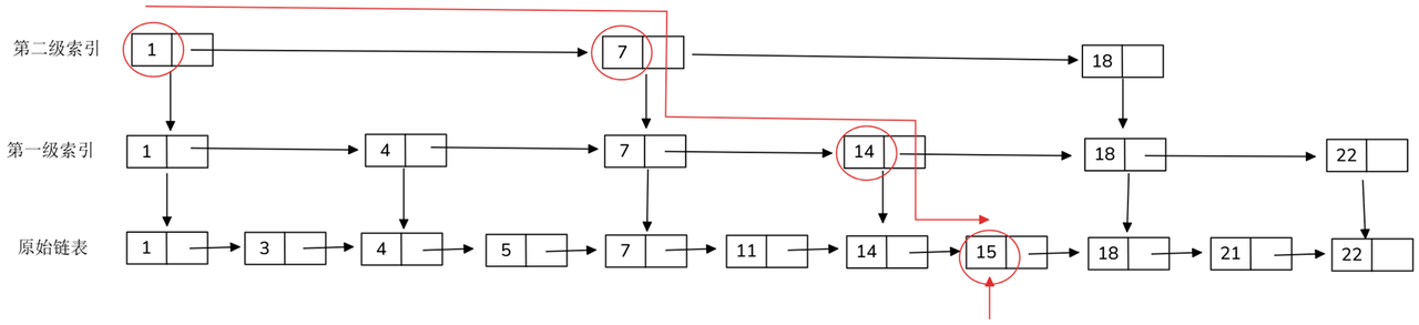
The jump list consists of a multi-level ordered linked list, with the bottom layer containing all nodes; from the bottom upward, each layer samples the "jump point" of the previous layer according to probability p (usually 0.25-0.5). This kind of probabilistic balancing allows the skip table to achieve performance similar to that of the balanced tree without the need for complex rebalancing. characteristic**:

• Average O(log N) queries, insertions, deletions - The expected path length is logarithmically related to the number of nodes.
• Simple implementation, local update - only need to adjust the adjacency pointer, very suitable for high concurrent writing.
• Naturally ordered - supports range scanning and positioning by rank. The underlying index of Redis ZSET is the skip table.

Vector Index

Vector index is an index structure used to accelerate high-dimensional vector data similarity retrieval. Its goal is to quickly find several vectors that are most similar (Top-K) to a certain query vector in large-scale data sets. Vector indexing is not just about storing data but also about intelligently organizing vector embeddings to optimize the retrieval process. At present, vector indexes basically use the ANN method. Commonly used vector index structures include IVF, PQ, HNSW, etc.

	Features and applicable scenarios
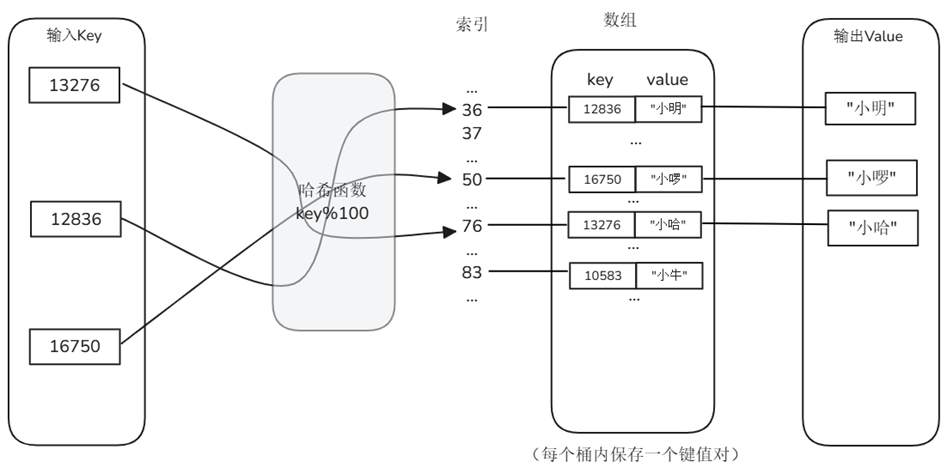
IVF (Inverted File Index)	First use clustering to divide the data into multiple "buckets". When querying, only perform local searches within a few relevant buckets, which is suitable for large-scale data (such as millions)
PQ (Product Quantization)	Compresses high-dimensional vectors into low-dimensional discrete codes to increase storage density and is suitable for memory-limited scenarios
HNSW (Hierarchical Navigable Small World)	Based on the graph structure, multiple hierarchical neighbor graphs are constructed. It is suitable for medium and high dimensions and has extremely fast query speed. It is one of the most mainstream ANN algorithms at present

KNN & ANN

​ For a RAG system, each vector retrieval can be described as "Given the query vector q, find several vectors with the smallest (or largest) distance (or similarity) in the vector set V." This process is called Nearest Neighbor (NN). In the previous RAG practical course, we introduced the similarity calculation index (Similarity) of vectors. Taking cosine similarity as an example, if we expect to use cosine similarity for nearest neighbor search, the process is to calculate cosine similarity one by one for the vectors in the database, and finally find the data most similar to the target data from the database. When Top K exists in the retrieval parameters, that is, when the top K data items most similar to the target data need to be found, the above search process evolves into K-Nearest Neighbor (K-NN). However, when |V| reaches millions or even billions, the linear scan of calculating similarities one by one becomes time-consuming and difficult to scale.

For the above reasons, current vector retrieval usually uses the Approximate Nearest Neighbor (ANN) search algorithm. By pre-building vector indexes, the query phase only accesses a subset of the vector space, using less distance calculations in exchange for the approximately optimal solution, thereby performing efficient vector retrieval at the expense of a certain degree of accuracy and improving the user experience of the system. This idea of ​​“trading precision for speed” is especially useful when dealing with large, high-dimensional data sets, as it can drastically reduce search time while still maintaining high result quality.

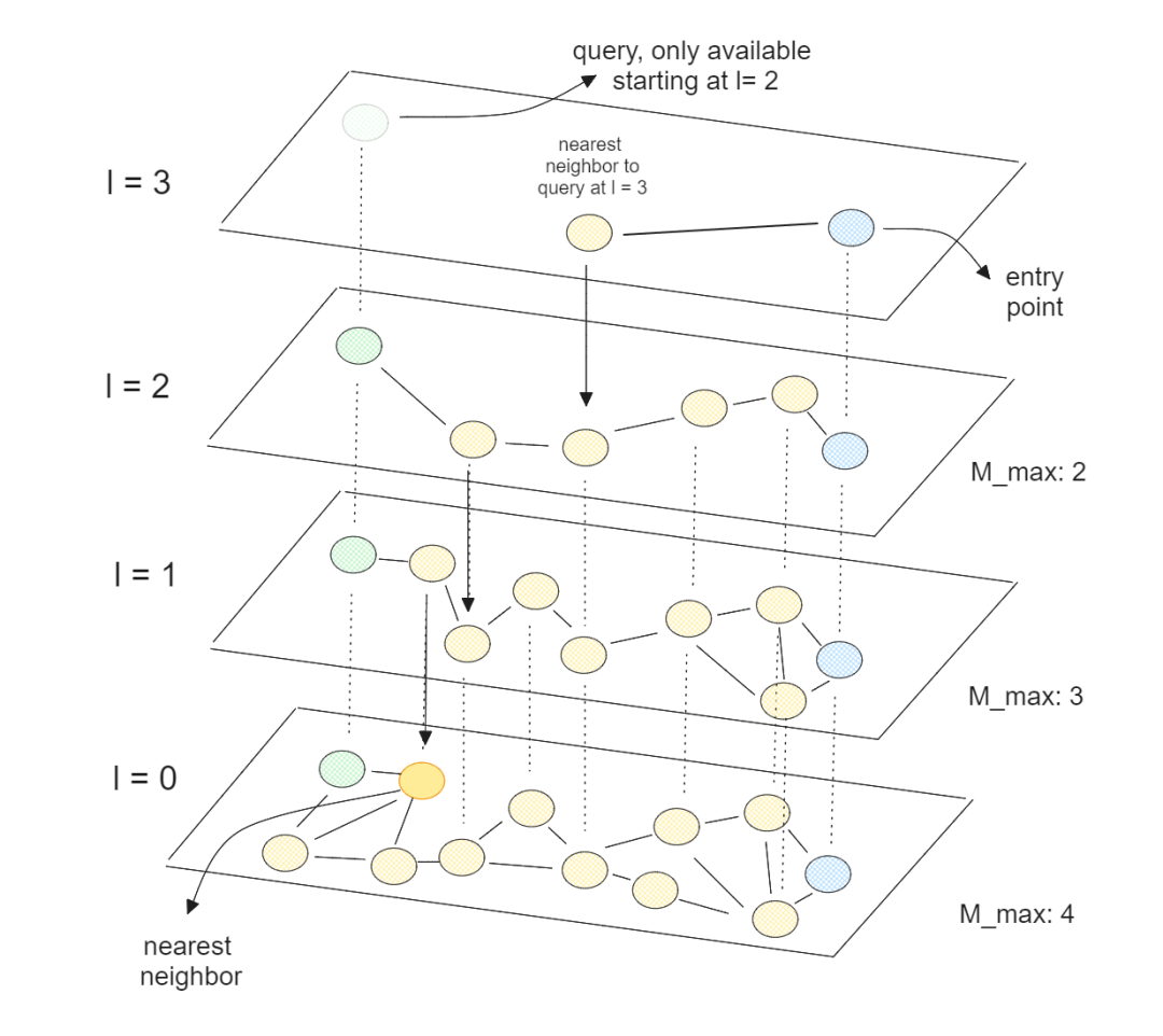
Let’s take the commonly used vector index type HNSW (Hierarchical Navigable Small World, Hierarchical Navigable Small World) as an example:

• Multi-layer graph structure: In the construction phase, vectors are randomly assigned to multiple layers L ~ 0 according to distance. Small layers contain all vectors, and large layers only sample a small number of "representative points" to form a pyramid.
• Top random starting point: The query vector enters the highest level, and any node is selected as the starting point.

• Greedy Neighbor Jump: Repeatedly executed in the current layer:

  • Calculate the distance between the current node's neighbors and the query vector;
  • Select the nearest neighbor;
  • If the neighbor is closer than the current node, jump to it and continue, otherwise stop (reach local optimal).
  • Downward layer by layer: Use the "local nearest node" as the entrance to the next layer, and proceed layer by layer until the bottom layer 0, and find the nearest neighbor.

Through the above query algorithm, there is no need to retrieve elements with low similarity that are far away from the query point, thereby increasing the retrieval efficiency (at the same time, HNSW finds an approximately optimal solution). The time complexity of HNSW is \(O(logN)\).

Therefore, in the RAG system, the vectors obtained from the Embedding model are combined with document slices and metadata to form a node set, and a vector index based on ANN is constructed, which can greatly reduce the calculation amount of the retrieval process and improve the response speed of the retrieval phase of the RAG system.

• Inverted File (IVF)

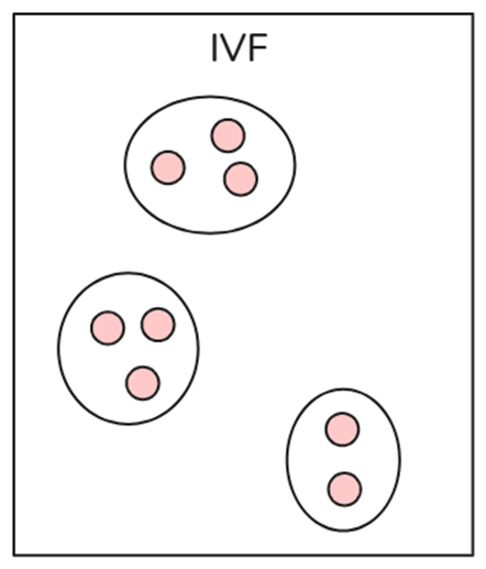
IVF is the most basic indexing technology in vector indexing, which uses techniques such as K-means clustering to divide the entire data into multiple clusters. Each vector in the database is assigned to a specific cluster. This structured arrangement of vectors enables users to conduct search queries faster. When a new query occurs, the system does not traverse the entire data set. Instead, it identifies the nearest or most similar clusters and searches for specific documents within those clusters. IVF only performs brute force searches within relevant clusters instead of searching in the entire database, thereby increasing search speed and reducing query time.

• Product Quantization (PQ)

Product quantization is an efficient vector compression and nearest neighbor search (ANN) method, especially suitable for high-dimensional data. It reduces storage overhead and accelerates nearest neighbor search by decomposing high-dimensional vectors into multiple subspaces and quantizing each subspace separately.

The core stages of PQ are divided into: training, quantification, query

Training: Divide the high-dimensional vector into M segments, and perform K-means clustering on each segment in the training set. Assuming K=256, each segment has 256 center vectors.

Quantification: With K cluster center vectors, they can be numbered, for example, ClusterID=0~255.

Query:

The query vector is segmented according to the same rules, and the distance between each segment and the K cluster centers of the segment is calculated to form a distance table (M*K).

Iterate over the candidate vectors and calculate the sum of the distances in the distance table.

Select the most similar topk vectors.

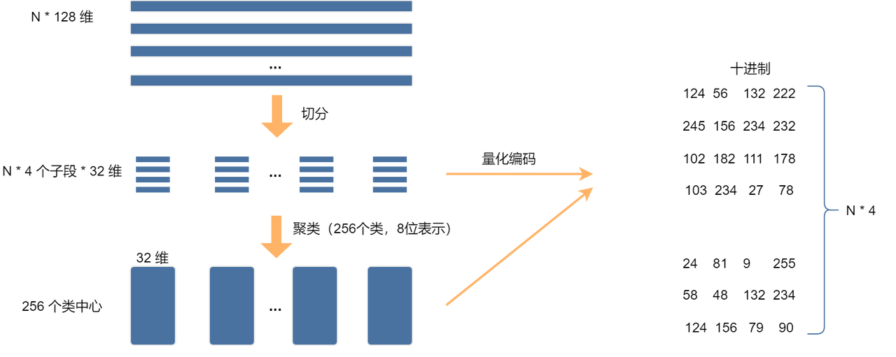
The above figure shows the process of the PQ algorithm. Assume that there are N 128-dimensional vectors, which are divided into 4 subspaces. The feature dimension of each subspace is 32, and then k-means clustering is performed in each subspace. The eight-bit representation means that the storage space occupied is 1/128 of the original, which greatly reduces the storage space. After quantized encoding, a lot of calculations will be saved when querying. Let's look at a simple example to experience it. Suppose we have the following 4-dimensional vector:

X1=[3.2,4.5,1.8,2.7]

X2=[2.9,4.3,1.5,2.9]

X3=[3.1,4.6,1.9,2.5]

X4=[3.0,4.4,1.7,2.8]

Suppose we split the 4-dimensional vector into 2 2-dimensional sub-vectors, we can get:

First part (first 2 dimensions): [3.2, 4.5], [2.9, 4.3], [3.1, 4.6], [3.0, 4.4]

Second part (last 2 dimensions): [1.8, 2.7], [1.5, 2.9], [1.9, 2.5], [1.7, 2.8]

Perform K-Means clustering on each subspace (assuming there are 2 clustering centers. In practice, this clustering center needs to be obtained through training), then the clustering center of the first subspace can be obtained as: \(C1_1 = [3.0, 4.4], C1_2 = [3.2, 4.5]\), and the clustering center of the second subspace is: \(C2_1 = [1.8, 2.7], C2_2 = [1.5, 2.9]\).

The closest subspace index for X1 = [3.2, 4.5, 1.8, 2.7] is: \((C1_2, C2_1)\). So we can encode X1 with the index (2, 1) instead of storing a full 4-dimensional floating point number.

Suppose we have a query vector Q=[3.1,4.5,1.7,2.8], split the query vector into [3.1, 4.5] and [1.7, 2.8], and then calculate the distance from the cluster center. Taking the first subspace as an example, there is:

\[d_{Q-C1_1}=\sqrt{(3.1 - 3.0)^2 + (4.5 - 4.4)^2} \\ = \sqrt{0.01 + 0.01}\\ = \sqrt{0.02}\approx 0.14\]

Calculated in the same way, \(d_{Q-C1_2}=0.1, d_{Q-C2_1}=0.14, d_{Q-C2_2}=0.22\) are obtained respectively. The quantization index is (2,1), which matches X1 and X3. Then \(d_{Q-X1}\) and \(d_{Q-X3}\) are calculated, and 0.17 and 0.37, and the closest matching vector is X1.

The overall query complexity of product quantization is \(O(m⋅k+n⋅m)\), where m is the number of subspaces, k is the cluster center, and n is the total amount of data, usually k=256. When n reaches the million/billion level, PQ is faster than brute force search. It can further be combined with the inverted index (IVF-PQ) to accelerate the query, making the query time sublinear; when d reaches 512 dimensions, PQ can effectively reduce storage costs. However, PQ will also affect accuracy due to the reduction of information in each subspace due to splitting high-dimensional data. In addition, PQ relies on k-means clustering, and if the cluster center is poorly selected, the error may be large.

• Hierarchical Navigable Small World (HNSW)

HNSW (Hierarchical Neighbor Small World) is a graph indexing method that divides graphs into multiple levels. It is a commonly used index in vector databases. The higher the level, the fewer the corresponding nodes. Start searching from high-level points, and search step by step to finally find the target node. The following figure is a simple example. After constructing the hierarchical graph as shown in the figure, the search starts from the blue point 0, and finds the green point 1 that is closer to the query in layer 2. At this time, layer 2 has no other points, so it searches layer 1, finds point 2 in layer 1, and finally finds point 3 in layer 0, which effectively reduces the total amount of calculations.

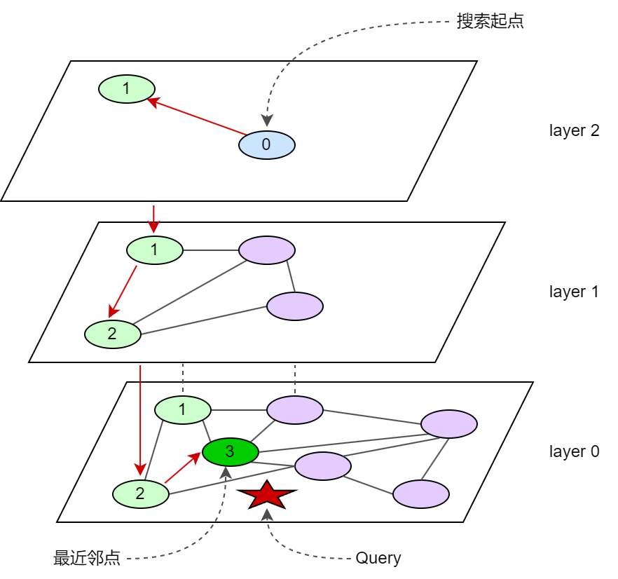
HNSW retrieval time complexity is typically O(log n), where n is the number of elements in the dataset. Its hierarchical structure enables the search to start from the top layer and gradually refine it to the lower layers. The number of nodes in each layer decreases exponentially, thus greatly reducing the search path length. In each layer, the algorithm takes advantage of the "small world network" characteristics" (i.e., high clustering and short paths) to quickly locate candidate nodes through a greedy strategy, avoiding global traversal. The complexity of each layer search is constant time, and the number of layers is O(log n), so the overall complexity is O(log n). Therefore, HNSW is suitable for fast approximate nearest neighbor search for large-scale high-dimensional data.

2.4.2 High-performance vector database Milvus

In enterprise-level RAG system scenarios, there are sometimes millions or even hundreds of millions of data scale. At the same time, there may be some special condition restrictions based on vector retrieval (such as document date, language, author attribute filtering). The high-performance vector database Milvus can easily handle these complex storage and retrieval requirements, which is why LazyLLM is deeply adapted to it.

Milvus system architecture

Milvus' cloud-native and highly decoupled system architecture ensures that the system can continue to scale as data grows:

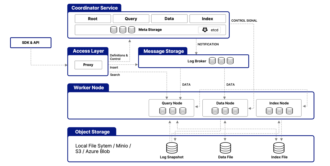
Milvus itself is completely stateless, so it can be easily scaled with Kubernetes or the public cloud. In addition, the various components of Milvus are well decoupled, with the three most critical tasks - search, data insertion and indexing/compaction - being designed as easily parallelizable processes, with complex logic separated. This ensures that corresponding query nodes, data nodes, and index nodes can be scaled up and down independently, optimizing performance and cost efficiency.

In addition, Milvus offers three deployment modes covering various data sizes - from on-premises prototypes to large-scale Kubernetes clusters managing tens of billions of vectors:

• Milvus Lite is a Python library that can be easily integrated into your application. As a lightweight version of Milvus, it is ideal for rapid prototyping in Jupyter Notebooks or running on edge devices with limited resources.
• Milvus Standalone is a stand-alone server deployment, and all components are bundled in a Docker image for easy deployment.
• Milvus Distributed can be deployed on Kubernetes clusters, adopts cloud-native architecture, and is designed for scenarios with a scale of one billion or more. The architecture ensures redundancy of critical components.

Why can Milvus achieve fast retrieval?

The high performance of Milvus benefits from the following points:

• Hardware Aware Optimization: In order to adapt Milvus to various hardware environments, its performance is optimized for multiple hardware architectures and platforms, including AVX512, SIMD, GPU and NVMe SSD.
• Advanced Search Algorithms: Milvus supports multiple memory and disk indexing/search algorithms, including IVF, HNSW, DiskANN, etc., all of which are deeply optimized. Milvus achieves 30%-70% performance improvements compared to popular implementations such as FAISS and HNSWLib.
• C++ Search Engine: More than 80% of a vector database's performance depends on its search engine. Milvus uses C++ for this key component due to the language's high performance, low-level optimizations, and efficient resource management. On top of that, Milvus integrates a host of hardware-aware code optimizations, from assembly-level vectors to multi-threaded parallelization and scheduling, to take full advantage of hardware capabilities.
• Column-oriented: Milvus is a column-oriented vector database system. Its main advantage comes from the data access model. When executing a query, column-oriented databases only read the specific fields involved in the query rather than the entire row, which greatly reduces the amount of data accessed. Additionally, operations on column-based data can be easily vectorized, allowing operations to be applied across an entire column at once, further improving performance.

Scalar filtering

When performing vector retrieval in Milvus, you may want to filter by some scalar fields (for example, numerical values, string fields) to achieve more precise search results. For example, in image retrieval, you can filter results based on a scalar field such as the date the image was uploaded. However, the efficiency of scalar field filtering directly affects the speed of the final query. In order to solve this bottleneck, Milvus introduced scalar field index, which can effectively organize the data of scalar fields, and combined with inverted index, automatic indexing and other technologies, greatly improves query efficiency.

3. Optimize model inference performance

The RAG system's ability to answer users' questions based on external documents is mainly due to the development of large models. Generally speaking, the more model parameters there are, the greater the effect will be (for example, in the SuperCLUE open source model ranking list, the models ranked 4th and above all have parameter amounts of 30 billion and above, based on the December 2024 list). However, as the size of the model continues to increase, inference time (that is, the time for model prediction) has become a key factor affecting the system response speed and efficiency. Next, we will explore several methods to optimize the time of model inference, focusing on how to improve system performance by accelerating model inference based on software and hardware, as well as model quantization, model distillation and other technologies.

Inference acceleration based on software and hardware usually does not require developers to optimize on their own, and can often be achieved by replacing hardware and switching technical solutions.

3.1 Large model inference speed evaluation index

The goal of the large model inference service is to output the first token as quickly as possible, throughput as high as possible, and the time of each output token as short as possible, that is, the model service can support generating as much text for users as quickly as possible.

• TTFT (Time to First Token, first word delay): The time required from inputting the prompt word to the model to the model generating the first token.
• TPOT (Time Per Output Time): The delay of each output token of the model in the output stage (Decode).
• Throughput: Throughput, for model services, the number of tokens that the model service can process per unit time.
• BS (Batch Size): For model services, that is, the service combines and calculates the number of user requests (the method to improve throughput is generally to increase BS, but increasing BS will affect the delay of each user to a certain extent).

The main factors affecting the inference speed of large models are:

1. Calculation amount
   1. Model size (number of parameters) -> Distillation
   2. Use low-precision data
   3. Quantification
2. Computing performance
   1. Chip computing power
   2. Operator implementation
   3. Select an appropriate parallel strategy to optimize the interconnection between cards
   4. Choose a good reasoning framework

3.2 Hardware acceleration

In modern AI applications, GPUs, TPUs, and dedicated AI acceleration chips are key tools for improving inference speed. For large model inference, it usually involves hundreds of millions of parameters and complex mathematical operations, including a large number of floating point operations, such as matrix multiplication and nonlinear activation functions. These operations have high requirements on calculation accuracy and speed. The CPU we use daily in personal laptops, etc. is suitable for general tasks. It has fewer cores and is suitable for sequential execution of tasks. GPU, TPU, etc. are hardware specially designed for parallel computing. Take GPU as an example. It has thousands of small cores and can perform a large number of simple calculations at the same time. It is very suitable for matrix operations. Therefore, deep learning inference is faster and it is currently the mainstream AI computing hardware. In addition, support for deep learning frameworks is also an important reason. GPU/TPU has a powerful software ecosystem, including deep learning frameworks and libraries, such as CUDA, which provide optimized algorithms and APIs for these hardware, making the development of large models easier and more efficient. Therefore, the price of GPU/TPU is more expensive than that of CPU, and the computing performance of different types of GPU/TPU is also quite different. In particular, large model inference tasks have higher hardware requirements, requiring larger video memory and higher computing efficiency. Therefore, how to perform efficient large model inference based on limited hardware resources is also one of the current research hotspots.

3.3 Software acceleration

Software acceleration mainly improves reasoning efficiency by optimizing calculation methods, reducing redundant operations, and making full use of hardware parallelism. In recent years, with the development of large models, technologies and frameworks specifically designed for inference optimization have continued to emerge. The following are several typical software acceleration solutions:

(1) Flash Attention: Flash Attention is a technology that optimizes attention (Attention) calculation in the Transformer model. It is specially used to reduce video memory usage and accelerate reasoning. Traditional attention calculation creates a complete attention matrix, which requires a lot of graphics memory and computing resources. Flash Attention uses memory read and write optimization and parallel computing to avoid unnecessary memory accesses, thereby speeding up inference. Overall, Flash Attention reduces GPU memory usage, allowing larger models to be inferred on GPUs with limited memory. The inference speed is increased by 5-9 times compared to standard Attention, and it can also reduce video memory consumption.

(2) vLLM (Very Large Language Model Inference): VLLM is a framework that specifically optimizes large model inference and is suitable for Transformer models. VLLM further optimizes video memory management through Paged Attention, which enables more effective use of GPU memory during inference, reduces repeated calculations, and improves the speed of long text inference. In addition, VLLM supports parallel batch processing and parallel reasoning for multiple requests, thereby improving throughput. VLLM allows larger models to run under the same GPU resources. Using Continuous Batching technology to improve the inference efficiency of the same model can be increased by up to 23 times [data source and VLLM official documentation], which is suitable for scenarios that need to handle a large number of requests. Similar frameworks include LightLLM, LMDeploy, etc.

The above solutions are all software acceleration methods proposed for specific hardware. Usually, framework developers will adapt most models. Users only need to download the corresponding model weights and use the corresponding libraries to achieve accelerated inference effects. Although these methods can accelerate model inference, the number of parameters of the model itself has not decreased or changed. Models with better results are still tens of billions in size and still require a lot of hardware support. Therefore, we will introduce two technologies below to reduce dependence on a large amount of hardware while retaining model capabilities.

3.4 Model Quantification

Model quantization is a technique that reduces the storage requirements and computational overhead of a model by converting floating point weights in the model to lower precision numeric values ​​(for example, from 32-bit floating point numbers to 8-bit integers). By converting high-precision weights into lower-precision values, model quantization can significantly compress the model volume, reduce the amount of calculation and memory usage, greatly improve the inference speed on hardware that supports low-precision instructions, and reduce bandwidth overhead in distributed scenarios, allowing large models to run efficiently on resource-constrained devices.

Common quantization methods include: weight quantization, which converts the weights of the model from 32-bit floating point numbers to 8-bit integers or even 4-bit integers; activation quantization, which quantifies the activation values ​​of the neural network to further reduce computing resource requirements.

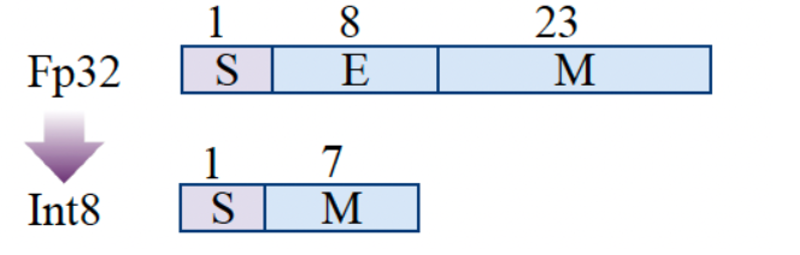
Common quantization precisions include INT8, INT4, etc. Through quantification, both the generation model and the retrieval model in the RAG system can significantly improve the inference speed and reduce the memory usage, thereby speeding up the overall system response time. In practice, you may see the specifications of various quantization models such as W8A8, W4A16, where W represents weight and A represents activation. Then W8A8 represents that both weight and activation are 8-bit integers. Currently commonly used large model quantification methods include GPTQ, AWQ, etc. The following is a brief introduction to AWQ to give you a preliminary understanding of model quantification technology. In actual practice, there are libraries such as AutoGPTQ and AutoAWQ that can be directly called to implement these quantification operations.

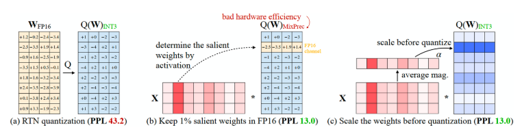
AWQ (Activation-aware Weight Quantization for LLM Compression and Acceleration) is a commonly used quantification technology. Its principle protects more "important" weights from quantification. The standard quantification process in deep learning is to quantize all weights from FP16 -> INT3/4, but AWQ believes that the weights of large language models are not equally important. There are a small number of key weights (salient weights) that have a far greater impact on model performance than other weights. If the quantization of these key weights is skipped during the quantization process, the performance degradation caused by the quantization loss can be mitigated without additional training or regression (i.e., (b) above). However, this approach will lead to low hardware efficiency due to different precisions. AWQ proposes a method to reduce the quantization error of significant weights through channel-by-channel scaling (as shown in (c) above), which can effectively circumvent hardware efficiency issues. Specifically, before performing weight quantization, the channel weight is calculated, that is, the average amplitude (magnitude) of each channel. After obtaining this weight, the channel is scaled, and then the quantization step is performed. AWQ therefore does not rely on any regression or backpropagation, requires less data during quantization, and can preserve the knowledge of the LLM outside the calibration set distribution.

According to the data provided in the AWQ quantization method paper, the model quantized using AWQ is 3 times faster than the FP16 model under the same circumstances, and reduces the memory requirements by 3 times. Taking the AWQ quantified Qwen-72B model as an example, the average differences between the two in MMLU, C-EVAL, and IFEval are 0.9, 81.3 and 80.4 respectively, but the hardware requirements are 144GB and 48GB respectively. It can be seen that the quantized model can save a lot of video memory requirements while retaining the higher accuracy of the original model.

In the model open source community, developers can easily obtain a large number of excellent quantitative models.

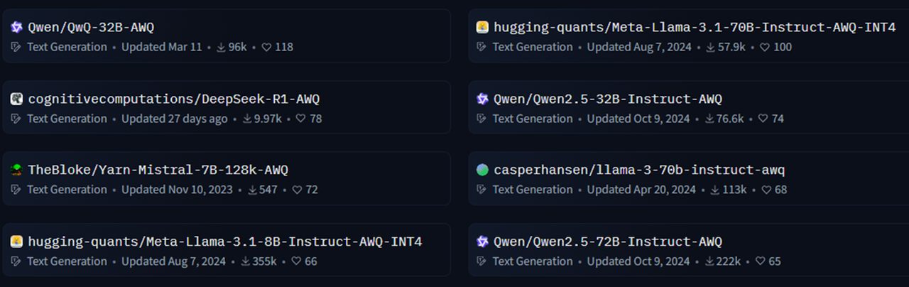
3.5 Model Distillation

As the scale of deep learning models continues to grow, the consumption of computing resources and inference time also increases significantly. Model distillation (Knowledge Distillation, KD) as a model compression technology can transfer the knowledge of large and complex models into smaller models without significantly sacrificing model performance, making inference more efficient and easier to deploy. This technique was first proposed by Hinton et al. in 2006 and further systematized in 2015. In recent years, with the rise of large language models (LLM), they have been widely used in many fields.

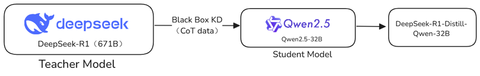
The core idea of ​​model distillation is to use a large model with high accuracy (Teacher Model) to guide a smaller model (Student Model) to learn, so that it can achieve performance close to that of the teacher model at a lower computational cost. Compared with directly training a small model, the student model can learn the knowledge structure of the teacher model during the distillation process, making it have stronger generalization capabilities. A typical example is DistilBERT, which is a model distilled from BERT-base. It is only 40% of the size of the original model, but can maintain 97% of the performance while increasing the inference speed by 60% (data from the DistilBERT paper). This case fully illustrates the important role of model distillation in optimizing inference efficiency.

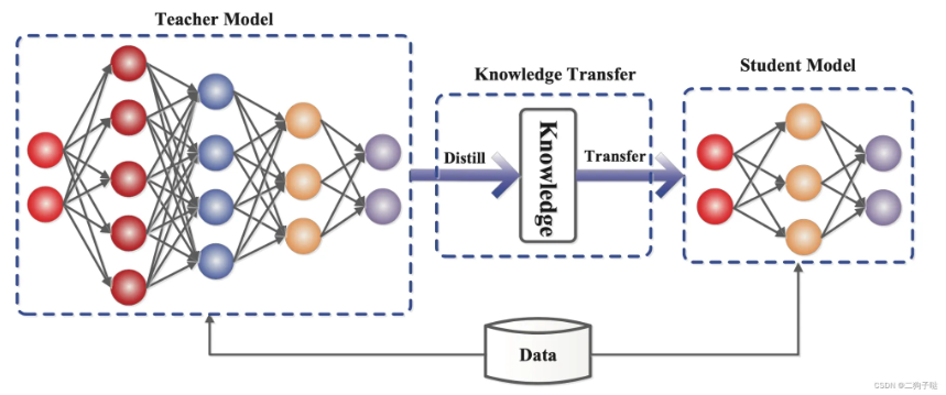
Generally, knowledge distillation methods can be divided into two categories:

(1) Black-box Knowledge Distillation: In the black-box distillation mode, the teacher model is regarded as an inaccessible black box, and we can only obtain its final output. The student model is trained by having it imitate the output of the teacher model and optimizing the parameters of the student model by minimizing the gap between the two. This method is computationally cheap, but the distillation effect is usually not as good as white-box distillation due to the lack of internal information of the teacher model.

(2) White-box Knowledge Distillation: In the white-box distillation mode, in addition to the final output, information such as hidden layer features, intermediate representations and even attention mechanisms of the teacher model are also accessible. The student model not only needs to learn the output distribution of the teacher model, but can also further narrow the gap with the teacher model by imitating its middle layer features, attention matrix, etc. White-box distillation often achieves better performance but requires more sophisticated training methods.

Lightweight reasoning can be achieved through knowledge distillation. Large models (such as GPT-4, DeepSeek) usually have huge parameters and require parallel computing on multiple GPUs during inference. However, the distilled model can be inferred on a single GPU or even a CPU, significantly reducing deployment costs. For example, DeepSeekR1 (671B) requires 16 80G graphics cards to deploy inference services, but through knowledge distillation, taking the 7B model as an example, it only requires 14G graphics memory.

Although knowledge distillation has many advantages, there are still certain challenges in practical applications. For example, because the capacity of the student model is smaller than that of the teacher model, it may not be able to fully reproduce the capabilities of the teacher model. Compared to direct quantization or pruning, knowledge distillation requires additional training steps and requires the selection of an appropriate loss function. In addition, although the distilled student model infers faster, training or deploying a high-quality teacher model may still require a lot of computing power.

In practical applications, distillation and quantification can be used together. For example, distillation is used to obtain a small model and then quantized, thereby minimizing computational costs while ensuring accuracy. More details about model distillation will not be discussed in this section. Interested readers can jump to the elective content to learn the DeepSeekR1 distillation tutorial.

3.6 Model parameter accuracy

The training and inference of large models often involve the concept of accuracy. Higher accuracy is more accurate, but it also brings higher computing and storage costs. Lower precision reduces computational accuracy but improves computational efficiency and performance. So a variety of different accuracies allow you to choose the most suitable one in different situations.

Floating Point Precision (FP): The most primitive precision, consisting of sign bit (sign, positive/negative), exponent bit (exponent, indicating the range of the integer part), and mantissa bit (fraction, indicating the decimal part). Common precisions include FP64, FP32, and FP16 (FP8 and FP4 are not IEEE standard formats)

\[\text{value} = (-1)^s \times \text{1.f} \times 2^{e - \text{bias}} \\ \text{bias} = 2^{\text{bitlen}(e) - 1} - 1\]

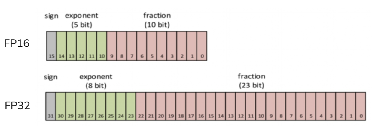
• TF32: TF32 (Tensor Float 32) is a special numerical type designed by NVIDIA for machine learning and is used to replace FP32. Supported for the first time in A100 GPU. It consists of 1 sign bit, 8 exponent bits (aligned to FP32) and 10 decimal bits (aligned to FP16). There are actually only 19 bits. A balance of performance, range and precision.

import torch
//Whether tf32 is supported
torch.backends.cuda.matmul.allow_tf32
//Whether tf32 is allowed, the default is False in PyTorch1.12 and higher versions
torch.backends.cudnn.allow_tf32

• BF16: BF16 (Brain Float 16) was proposed by Google Brain and is also designed for machine learning. It consists of 1 sign bit, 8 exponent bits (consistent with FP32) and 7 decimal places (lower than FP16). Therefore, the accuracy is lower than FP16, but the representation range is consistent with FP32, and it is easy to convert between FP32 and FP32.

import transformers
transformers.utils.import_utils.is_torch_bf16_gpu_available()

• FP8: FP8 is a data representation method unique to H100 and later graphics cards. Currently, almost no domestic cards have this format. There are two common variant formats, E4M3 and E5M2.

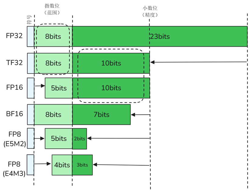
3.7 Parallel Strategy

Tensor Core

Tensor Core is a hardware acceleration unit that NVIDIA GPU only has in A100 and later. Compared with traditional CUDA Core, Tensor Core can process more data in parallel in one operation, thus greatly improving the speed of Matrix Multiplication (GEMM) and making deep learning training more efficient.

	CUDA Core	Tensor Core
Main purposes	General computing (GPGPU)	AI training & inference
Supported data types	FP32, INT32, etc.	FP16, TF32, INT8, INT4, FP64, etc.
Performance Features	Strong versatility, supports various parallel computing tasks	Dedicated hardware acceleration, up to 16 times improvement, higher throughput
Typical Applications	Graphic rendering, scientific computing, high-performance computing	Deep learning model training and inference

CUDA acceleration

CUDA (Compute Unified Device Architecture) is a parallel computing platform and programming model provided by NVIDIA, which allows developers to use a language similar to C/C++ to perform general computing on GPU (ie GPGPU: General-Purpose computing on Graphics Processing Units)

• Parallel computing: GPU has thousands of cores, and CUDA distributes computing tasks to a large number of threads, allowing a large number of computing tasks to be completed instantly
• Efficient memory management: CUDA provides shared memory, global memory and other mechanisms to make memory access as parallel and high-speed as possible
• Tensor operation optimization: Many deep learning libraries (such as PyTorch) use CUDA to implement high-performance matmul, conv, norm and other operations at the bottom layer
• Automatically call the GPU: If the framework supports CUDA, it can automatically move the data to the GPU, use the CUDA core to calculate, and then return the results -Support mixed precision computing (Tensor Core): On new generation GPUs, CUDA can call Tensor Core to accelerate calculations with low precision such as float16 or int8, with almost no loss of model accuracy.

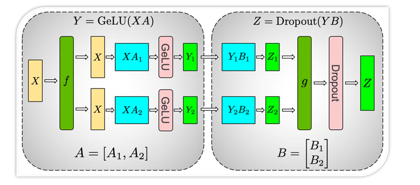
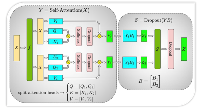
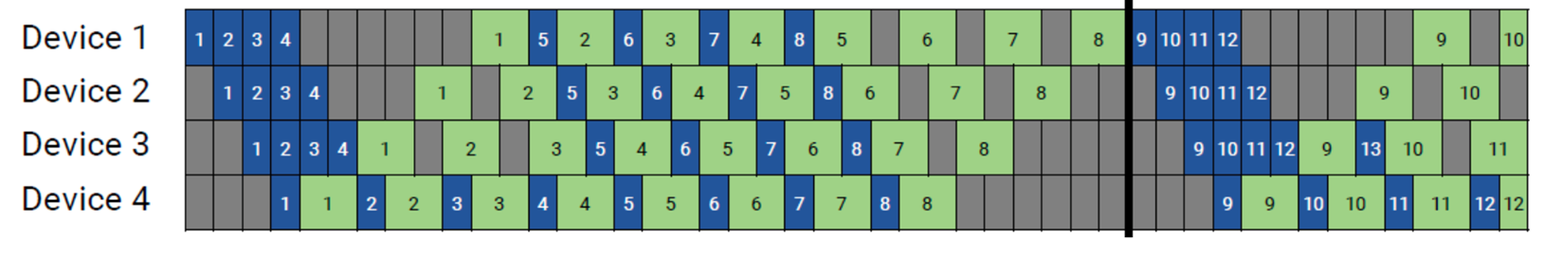
3.8 Sparse model structure – MoE

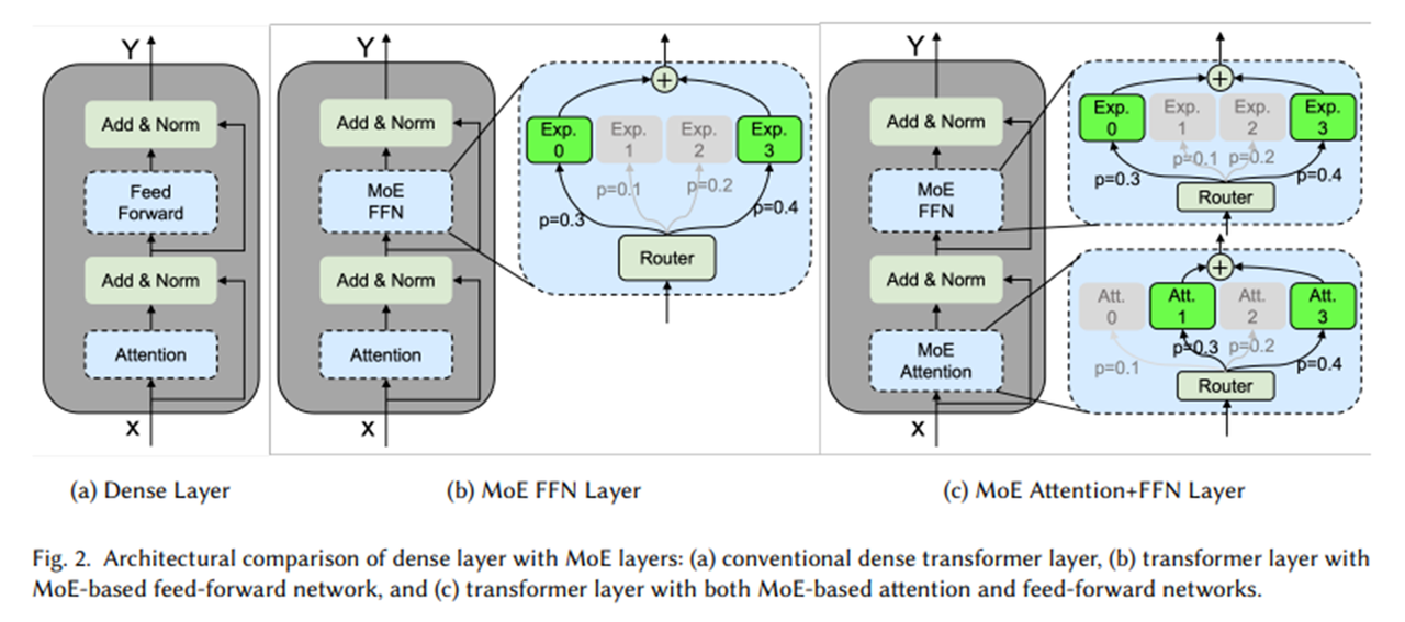
3.9 Better reasoning framework

When the model remains unchanged, the inference performance of large models can also be improved by choosing a better inference framework. The current mainstream model inference frameworks include Ollama, LightLLM, vLLM, LMDeploy, etc.

• Ollama
  • Pre-packaged models: Built-in LLaMA, Mistral and other models.
  • Strong hardware adaptability: CPU and GPU inference are optimized for daily use hardware, whether it is MacBook, PC or edge devices, it can run AI models smoothly.
  • Easy to operate: Provides a simple API and CLI, and can quickly start a large language model with simple configuration.
• LightLLM -Lightweight design: takes up less resources, is easy to deploy and expand, and makes it easy to get started quickly for local deployment and customized modifications.
  • High performance: Through a variety of optimization technologies such as three-process asynchronous collaboration, Token Attention, etc., high-speed reasoning is achieved and higher throughput is obtained.
  • Ease of use: Docker containers and detailed documentation are provided to simplify the use process and lower the barriers to use.
• vLLM
  • PagedAttention technology: breaks through the traditional KV cache mechanism, realizes video memory paging management, and supports the generation of ultra-long sequences (such as 100,000 token conversations).
  • Leading throughput: The A100 GPU can achieve more than 3 times the throughput of traditional frameworks and supports dynamic batch processing.
  • Ecological compatibility: natively supports the HuggingFace model format and is compatible with the PyTorch ecosystem.
• LMDeploy
  • Turbomind engine: using asynchronous pipeline parallelism, the delay is reduced to 50ms level
  • Quantitative deployment tool chain: supports W4A16 quantification, and model volume is compressed 4 times
  • Dynamic batch processing: intelligently merge requests of different lengths, GPU utilization reaches 90%+

LazyLLM has completed the perfect adaptation of the three frameworks of LightLLM, vLLM, and LMDeploy. Developers can flexibly choose the inference framework according to their actual needs to achieve the model inference experience that best suits them.

	Ollama	LightLLM	vLLM	LMDeploy
Core advantages	Personal PC running LLM	Lightweight, minimalist deployment	High concurrency processing	Domestic high-performance framework
Applicable scenarios	PC/smaller model	Personal debugging/prototype development	Enterprise-level service deployment	Domestic deployment plan
Hardware requirements	MacBook, PC, edge devices can run	Mid-range graphics cards can also run	NVIDIA high-performance graphics cards are required	Mid-range graphics cards can also run
Open Source License	MIT	Apache 2.0	Apache 2.0	Apache 2.0

3.10 Device-side reasoning framework

Device-side reasoning framework	Main features	Typical application chips
MLC LLM	Multi-backend compilation (WebGPU, Metal, CUDA, Vulkan), one set of code to run on multiple platforms	Mobile phone (iOS/Android), browser, PC
llama.cpp	Inference engine written in pure C/C++, extremely compact, adaptable to CPU/Metal/AVX	PC CPU, Mac (M series), mobile terminal
GGML/GGUF	Format + quantitative inference library, used with llama.cpp	CPU priority (including embedded CPU)
Core ML Tools	Apple's official inference framework, optimized for Apple Silicon (M series, A series chips)	iPhone, MacBook, iPad
OpenVINO	Produced by Intel, optimized for x86 CPU / VPU / Movidius NPU reasoning	Edge computing, industrial control equipment
TensorFlow Lite (TFLite)	A client-side lightweight version of TensorFlow that supports quantization and hardware acceleration	Mobile phones, micro devices (Raspberry Pi, etc.)
ONNX Runtime Mobile	A lightweight version of runtime launched by ONNX, supporting mobile acceleration	Android, iOS

Summarize

Building an efficient RAG system requires optimization at multiple levels to improve response speed and operating efficiency. The optimization of startup time can reduce the overhead of data loading and index construction through persistent storage, and combine with the caching mechanism to reduce repeated calculations, thus speeding up the secondary startup time of the system. Runtime retrieval speed is crucial to overall performance. Using an efficient vector database (such as Milvus) can improve vector retrieval efficiency, and at the same time, combined with technologies such as keyword indexing or inverted indexing, can further reduce query delays. In terms of model inference, quantification technologies (such as GPTQ, AWQ) can reduce the computational burden and increase the speed of inference, while knowledge distillation can transfer the knowledge of large models to smaller models, allowing them to maintain high performance while reducing computational costs. Combining these optimization strategies can significantly improve the stability and efficiency of the RAG system, making it more practical in practical applications.

References

Approximate neighbor graph: https://arxiv.org/pdf/2101.12631

HNSW：https://arxiv.org/abs/1603.09320

Flash Attention: https://arxiv.org/pdf/2205.14135

VLLM: https://docs.vllm.ai/en/latest/

AWQ：https://arxiv.org/pdf/2306.00978

DistillBERT：https://arxiv.org/pdf/1910.01108